Text Processing 📜¶

Despite the wealth of multimedia information, text processing remains one of the dominant functions of computers.

From Fluent Python - Unicode Text Versus Bytes:

Humans use text. Computers speak bytes.

1 - Esther Nam and Travis Fischer, Character Encoding and Unicode in Python

Abundance of Digitized Text¶

Computer are used to edit, store, and display documents, and to transport documents over the Internet.

Furthermore, digital systems are used to archive a wide range of textual information, and new data is being generated at a rapidly increasing pace.

A large corpus can readily surpass a petabyte of data (which is equivalent to a thousand terabytes (1 PB - 1000 TB), or a million gigabytes).

Common examples of digital collections that include textual information are:

• Snapshots of the World Wide Web, as Internet document formats HTML and XML are primarily text formats, with added tags for multimedia content

• All documents stored locally on a user’s computer

• Email archives

• Customer reviews

• Compilations of status updates on social networking sites such as Facebook

• Feeds from sites such as X and Tumblr

In this chapter we explore some of the fundamental algorithms that can be used to efficiently analyze and process large textual data sets.

In addition to having interesting applications, text-processing algorithms also highlight some important algorithmic design patterns.

Notations for Strings and the Python `str` Class¶

To allow fairly general notions of a string in our algorithm descriptions, we only assume that characters of a string come from a known alphabet, which we denote as Σ.

S = "CGTAAACTGCTTTAATCAAACGC"

For example, in the context of DNA, there are four symbols in the standard alphabet, Σ = {A, C, G, T}.

This alphabet Σ can, of course, be a subset of the ASCII or Unicode character sets, but it could also be something more general.

As it is a sequence, we can index and slice strings.

my_str = "sezai"
my_str_slice = my_str[2:0]  # this is None
bool(my_str_slice) # this is False

Prefix and Suffix¶

Tip

You'll probably see them a lot! They are simply the start and the end pieces of string 📜

In order to distinguish some special kinds of substrings, let us refer to any substring of the form S[0:k] for \(0 ≤k ≤n\) as a prefix of S; such a prefix results in Python when the first index is omitted from slice notation, as in S[:k].

Similarly, any substring of the form S[j:n] for \(0 ≤j ≤n\) is a suffix of S; such a suffix results in Python when the second index is omitted from slice notation, as in S[j:].

Here is an example:

# lets use S again
S = "CGTAAACTGCTTTAATCAAACGC"

my_prefix = "CGTAA"

my_suffix = "CGC"

prefix_to_all = "" # null strings are prefixs for all strings.
suffix_to_all = "" # null strings are suffixes for all strings.

Tip

Here is an important thing about stringappendlist - listappendforstrings:

Python Strings are immutable, so if you use += to append to an end of a string, you will make a lot of string instances, using memory.

Instead of that, use a list and later, join it's elements.

# do not do this
s = ""
for _ in range(5):
    s += "a"

# do this!
result = []
for _ in range(5):
    result.append("a")

final = "".join(result)

This is faster and more memory-efficient, especially for large strings.

Python Strings From Appendix A¶

Let's cover strings in detail with the help of the appendix! We already defined a string as a sequence of characters that come from some alphabet.

In Python, the built-in str class represents strings based upon the Unicode international character set, a 16-bit character encoding that covers most written languages.

Unicode is an extension of the 7-bit ASCII character set that includes the basic Latin alphabet, numerals, and common symbols.

Strings are particularly important in most programming applications, as text is often used for input and output.

A basic introduction to the str class was provided in Chapter 1.2.3, including use of string literals, such as "hello" , and the syntax str(obj) that is used to construct a string representation of a typical object.

Common operators that are supported by strings, such as the use of + for concatenation, were further discussed in Chapter 1.3.

This appendix serves as a more detailed reference, describing convenient behaviors that strings support for the processing of text.

To organize our overview of the str class behaviors, we group them into the following broad categories of functionality.

Searching Substrings¶

The operator syntax, pattern in s, can be used to determine if the given pattern occurs as a substring of string s.

Table A.1 describes several related methods that determine the number of such occurrences, and the index at which the leftmost or rightmost such occurrence begins.

Each of the functions in this table accepts two optional parameters, start and end, which are indices that effectively restrict the search to the implicit slice s[start:end].

For example, the call s.find(pattern, 5) restricts the search to s[5:].

Table A.1:

Calling Syntax	Description
`s.count(pattern)`	Return the number of non-overlapping occurrences of pattern
`s.find(pattern)`	Return the index starting the leftmost occurrence of pattern; else `-1`
`s.index(pattern)`	Similar to `find`, but raise `ValueError` if not found.
`s.rfind(pattern)`	Return the index starting the rightmost occurrence of pattern; else `-1`
`s.rindex(pattern)`	Similar to `rfind`, but raise `ValueError` if not found.

Using find might be safer, if you do not want to raise an Exception.

Strings in Python are immutable, so none of their methods modify an existing string instance.

However, many methods return a newly constructed string that is closely related to an existing one.

Table A.2 summarizes useful string methods. Some replace a pattern with another or change the case of characters.

Others handle text alignment or strip unwanted characters from the ends of a string.

Table A.2

Calling Syntax	Description
`s.replace(old, new)`	Return a copy of s with all occurrences of old replaced by new
`s.capitalize()`	Return a copy of s with its first character having uppercase
`s.upper()`	Return a copy of s with all alphabetic characters in uppercase
`s.lower()`	Return a copy of s with all alphabetic characters in lowercase
`s.center(width)`	Return a copy of s, padded to width, centered among spaces
`s.ljust(width)`	Return a copy of s, padded to width with trailing spaces
`s.rjust(width)`	Return a copy of s, padded to width with leading spaces
`s.zfill(width)`	Return a copy of s, padded to width with leading zeros
`s.strip()`	Return a copy of s, with leading and trailing whitespace removed
`s.lstrip()`	Return a copy of s, with leading whitespace removed
`s.rstrip()`	Return a copy of s, with trailing whitespace removed

Several of these methods accept optional parameters not detailed in the table.

For example, the replace method replaces all non overlapping occurrences of the old pattern by default, but an optional parameter can limit the number of replacements that are performed.

The methods that center or justify a text use spaces as the default fill character when padding, but an alternate fill character can be specified as an optional parameter.

Similarly, all variants of the strip methods remove leading and trailing whitespace by default, but an optional string parameter designates the choice of characters that should be removed from the ends.

Testing Boolean Conditions¶

Table A.3 includes methods that test for a Boolean property of a string, such as whether it begins or ends with a pattern, or whether its characters qualify as being alphabetic, numeric, whitespace, etc.

For the standard ASCII character set, alphabetic characters are the uppercase A–Z, and lowercase a–z, numeric digits are 0–9, and whitespace includes the space character, tab character, newline, and carriage return.

Conventions for what are considered alphabetic and numeric character codes are extended to more general Unicode character sets.

Calling Syntax	Description
`s.startswith(pattern)`	Return `True` if `pattern` is a prefix of string s
`s.endswith(pattern)`	Return `True` if `pattern` is a suffix of string s
`s.isspace()`	Return `True` if all characters of nonempty string are whitespace
`s.isalpha()`	Return `True` if all characters of nonempty string are alphabetic
`s.islower()`	Return `True` if there are one or more alphabetic characters, all of which are lowercased
`s.isupper()`	Return `True` if there are one or more alphabetic characters, all of which are uppercased
`s.isdigit()`	Return `True` if all characters of nonempty string are in 0–9
`s.isdecimal()`	Return `True` if all characters of nonempty string represent digits 0–9, including Unicode equivalents
`s.isnumeric()`	Return `True` if all characters of nonempty string are numeric Unicode characters (e.g., 0–9, equivalents, fraction characters)
`s.isalnum()`	Return `True` if all characters of nonempty string are either alphabetic or numeric (as per above definitions)

Splitting and Joining¶

Table A.4 describes several important methods of Python’s string class, used to compose a sequence of strings together using a delimiter to separate each pair.

Or to take an existing string and determine a decomposition of that string based upon existence of a given separating pattern.

This is important because you want to do operations on lists not repeatedly made strings:

Calling Syntax	Description
`sep.join(strings)`	Return the composition of the given sequence of strings, inserting sep as delimiter between each pair
`s.splitlines()`	Return a `list` of substrings of s, as delimited by newlines
`s.split(sep, count)`	Return a `list` of substrings of s, as delimited by the first count occurrences of sep. If count is not specified, split on all occurrences. If sep is not specified, use whitespace `" "` as delimiter.
`s.rsplit(sep, count)`	Similar to split, but using the rightmost occurrences of sep
`s.partition(sep)`	Return (head, sep, tail) such that s = head + sep + tail, using leftmost occurrence of sep, if any; else return (s, , )
`s.rpartition(sep)`	Return (head, sep, tail) such that s = head + sep + tail, using rightmost occurrence of sep, if any; else return ( , , s)

The join method is used to assemble a string from a series of pieces. An example of its usage is:

sentence = ' and '.join([ "red" , "green" , "blue" ]) 
print(sentence) # "red and green and blue"

Note well that spaces were embedded in the separator string.

In contrast, the command down below do not has any whitespace.

sentence_two = 'and'.join([ "red" , "green" , "blue" ]) 
print(sentence_two) # "redandgreenandblue"

The other methods discussed in Table A.4 serve a dual purpose to join, as they begin with a string and produce a sequence of substrings based upon a given delimiter.

For example, the call:

list_one = "red and green and blue".split(" and ")
print(list_one)  # [ "red" , "green" , "blue" ]

If no delimiter (or None) is specified, split uses white space as a delimiter; thus

list_two = "red and green and blue".split() # Uses whitespace as delimiter
print(list_two) # [ "red" , "and" , "green" , "and" , "blue" ].

String Formatting¶

The format method of the str class composes a string that includes one or more formatted arguments.

The method is invoked with a syntax s.format(arg0, arg1, ...), where s serves as a formatting string that expresses the desired result with one or more placeholders in which the arguments will be substituted.

As a simple example, the expression

my_string = '{} had a little {}'.format( "Mary" , "lamb" ) 
print(my_string) # "Mary had a little lamb"

The pairs of curly braces in the formatting string are the placeholders for fields that will be substituted into the result.

By default, the arguments sent to the function are substituted using positional order; hence, Mary was the first substitute and lamb the second.

However, the substitution patterns may be explicitly numbered to alter the order, or to use a single argument in more than one location.

For example, the expression is an interesting use case:

my_second_string = "{0}, {0}, {0} your {1}".format( "row" , "boat" ) 
print(my_second_string) # row, row, row your boat

All substitution patterns allow use of annotations to pad an argument to a particular width, using a choice of fill character and justification mode.

An example of such an annotation is "{:-^20}".format("hello").

In this example, the hyphen - serves as a fill character, the caret ^ designates a desire for the string to be centered, and 20 is the desired width for the argument.

formatted_text = "{:-^20}".format("hello") 
print(formatted_text) # -------hello--------

By default, space is used as a fill character and an implied < character dictates left-justification; an explicit > character would dictate right-justification.

There are additional formatting options for numeric types. A number will be padded with zeros rather than spaces if its width description is prefaced with a zero.

For example, a date can be formatted in traditional “YYYY/MM/DD” form as:

year = 2024
month = 1
day = 6
formatted_second_text = "{}/{:02}/{:02}".format(year, month, day)
print(formatted_second_text) # 2024/01/06

Integers can be converted to binary, octal, or hexadecimal by respectively adding the character b, o, or x as a suffix to the annotation.

The displayed precision of a floating-point number is specified with a decimal point and the subsequent number of desired digits.

For example, the expression is a precision tuning for a float value:

formatted_fourth_string = "{:.3}".format(2/3) 
print(formatted_fourth_string) # 0.667

A programmer can explicitly designate use of fixed-point representation (e.g., 0.667 ) by adding the character f as a suffix, or scientific notation (e.g., 6.667e-01 ) by adding the character e as a suffix.

a = 3.3e-1
print(a) # 0.33

Tip

f-strings are better - faster - stronger.

sel = 4.5676
rowie = 5
real_ten = 11
print(f"{sel:.2f}") # "4.57"
print(f"{real_ten} is not equal to 10. omg. {rowie} is 5 tho")

seq = [1,2,3,4]
set_mine = {1, 3, 5, 7}
a,b,c,d,e, *f = range(8)
print(f"{seq[1:2]} and {set_mine}") # [2] and {1, 3, 5, 7}

a,b, *c = range(8)

print(a) # 0

print(b) # 1

print(c) # [2, 3, 4, 5, 6, 7]

Pattern Matching Algorithms¶

In the classic pattern-matching problem, we are given a text string T of length n and a pattern string P of length m, and want to find whether P is a substring of T.

If so, we may want to find the lowest index j within T at which P begins, such that T[j:j+m] equals P, or perhaps to find all indices of T at which pattern P begins.

The pattern-matching problem is inherent to many behaviors of py’s str class, such as P in T , T.find(P), T.index(P), T.count(P), and is a sub task of more complex behaviors such as T.partition(P), T.split(P), and T.replace(P, Q).

Quick Workout:

my_str = "we_love_learning_it makes us grow!"

print(f"where is underscore? {my_str.find('_')}") # 2

print(f"where is l? {my_str.index('l')}") # 3

print(f"where is next l? {my_str.index('l', 4)}") # 8

print(f"how many e's are in my_str?: {my_str.count('e')}") # 4

# Partition the string into three parts using the given separator.
print(my_str.partition(" "))

# Return a list of the words in the string, using sep as the delimiter string.
print(my_str.split())

# Return a copy with all occurrences of substring old replaced by new.
print(my_str.replace("makes", "helps"))

would result in:

where is underscore? 2 
where is l? 3 
where is next l? 8 
how many e's are in my_str?: 4 
('we_love_learning_it', ' ', 'makes us grow!') 
['we_love_learning_it', 'makes', 'us', 'grow!'] 
we_love_learning_it helps us grow!

Another workout:

drake = "Tuscan Leather"

print(drake.find("L")) # 7

# start, end
print(drake.find("a", 0, 6)) # 4

print(drake.find("W")) # -1

print(drake.index("a")) # 4

print(drake.index("W")) # ValueError substring not found

print(drake.index("a", 5)) # 9

print(drake.lower().count("t")) # 2

print(drake.split()[1][2:4]) # at

print(drake.partition(" ")) # ('Tuscan', ' ', 'Leather')

In this section, we present three pattern-matching algorithms (with increasing levels of difficulty).

For simplicity, we model the outward semantics of our functions upon the find method of the string class, returning the lowest index at which the pattern begins, or −1 if the pattern is not found.

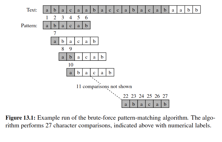
Brute Force - Pattern Matching¶

The brute-force algorithmic design pattern is a powerful technique for algorithm design when we have something we wish to search for or when we wish to optimize some function.

When applying this technique in a general situation, we typically enumerate all possible configurations of the inputs involved and pick the best of all these enumerated configurations.

def find_brute(T, P):
    """Return the lowest index of T at which substring P begins (or else -1)."""
    n, m = len(T), len(P) # introduce convenient notations
    for i in range(n - m + 1): # try every potential starting index within T
        k = 0 # an index into pattern P
        while k < m and T[i + k] == P[k]: # kth character of P matches
            k += 1 
        if k == m: # if we reached the end of pattern,
            return i # substring T[i:i+m] matches P
    return -1 # failed to find a match starting with any i

find_brute("Tuscan Leather" , "a") # 4
find_brute("Tuscan Leather" , "can") # 3

Two nested loops. Outer loop indexing through all possible starting indices of the a pattern of the text, inner loop indexing through each character of the pattern.

Outer loop executes at most \(o(n-m+1)\) - inner loop at most \(o(m)\). Worst case running time: \(O(n.m)\).

We run it again and again and again...

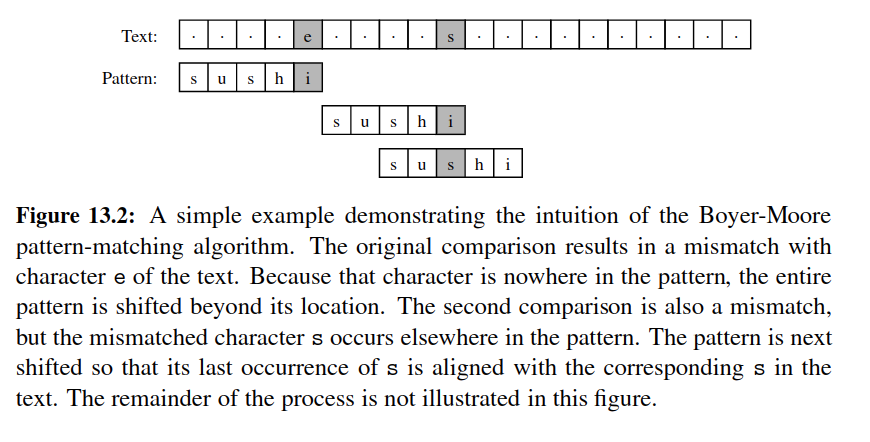
brute_force_example — Brute Force Visualized

Boyer Moore¶

Can we do it better?

At first, it might seem that it is always necessary to examine every character in T in order to locate a pattern P as a substring or to rule out its existence. But this is not always the case.

The Boyer-Moore pattern-matching algorithm, which we study in this section, can sometimes avoid comparisons between P and a sizable fraction of the characters in T.

Looking-Glass Heuristic: When testing a possible placement of P against T, begin the comparisons from the end of P and move backward to the front of P.
Character-Jump Heuristic: During the testing of a possible placement of P within T, a mismatch of text character T[i]=c with the corresponding pattern character P[k] is handled as follows. If c is not contained anywhere in P, then shift P completely past T[i] (for it cannot match any character in P). Otherwise, shift P until an occurrence of character c in P gets aligned with T[i].

We are likely to avoid lots of needless comparisons by significantly shifting P relative to T using the character-jump heuristic.

boyer_moore_pattern_matching — Boyer Moore Pattern Matching

The efficiency of the Boyer-Moore algorithm relies on making ==a lookup table== that quickly determines where a mismatched character occurs elsewhere in the pattern.

def find_boyer_moore(T, P):
    """Return the lowest index of T at 
    which substring P begins (or else -1)."""
    n, m = len(T), len(P) # introduce convenient notations
    if m == 0: return 0 # trivial search for empty string
    last = {} # build ’last’ dictionary
    for k in range(m):
        last[P[k]] = k # later occurrence overwrites

    # align end of pattern at index m-1 of text
    i = m - 1 # an index into T
    k = m - 1 # an index into P

    while i < n:
        if T[i] == P[k]: # a matching character
            if k == 0: 
                return i # pattern begins at index i of text
            else:
                i -= 1 # examine previous character
                k -= 1 # of both T and P 
        else:
            j = last.get(T[i], -1) # last(T[i]) is -1 if not found
            i += m - min(k, j + 1) # case analysis for jump step
            k = m - 1 # restart at end of pattern
    return -1

find_boyer_moore("alareference", "ref")  # 3

Here is a figure on it:

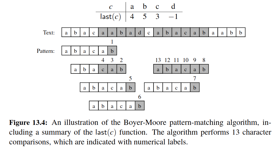
boyer_moore_illustrated — Boyer Moore Illustrated

Performance¶

If using a traditional lookup table, the worst-case running time of the Boyer-Moore algorithm is \(O(nm+ |Σ|)\).

Namely, the computation of the last function takes time O(m+ |Σ|), and the actual search for the pattern takes \(O(n*m)\) time in the worst case, the same as the brute-force algorithm (With a hash table, the dependence on |Σ| is removed.).

An example of a text-pattern pair that achieves the worst case is:

T = aaaaaaaaaaaa (n pieces)

P = baaaaaaaa (m-1 pieces of a)

The worst-case performance, however, is unlikely to be achieved for English text, for, in that case, the Boyer-Moore algorithm is often able to skip large portions of text.

Experimental evidence on English text shows that the average number of comparisons done per character is \(0.24\) for a five-character pattern string.

Tip

For quicksort, the worst-case time complexity is \(O(n^2)\) when the pivot selection consistently results in poor partitioning. However, on average and in practice, quicksort tends to perform very well and often outperforms algorithms with better worst-case time complexities.

Similarly, the Boyer-Moore algorithm has a worst-case time complexity of \(O(nm + |\Sigma|)O(nm+∣Σ∣)\), but its typical performance on English text (or other real-world scenarios) is much better.

The algorithm is designed to efficiently skip large portions of text during the search, making it particularly effective in practice, especially for long texts and relatively short patterns.

In both cases, the worst-case scenario is less likely to occur in typical real-world applications, and the algorithms can exhibit superior performance in practice. Experimental evidence and empirical analysis on representative data sets help provide a more accurate understanding of their average-case behavior.

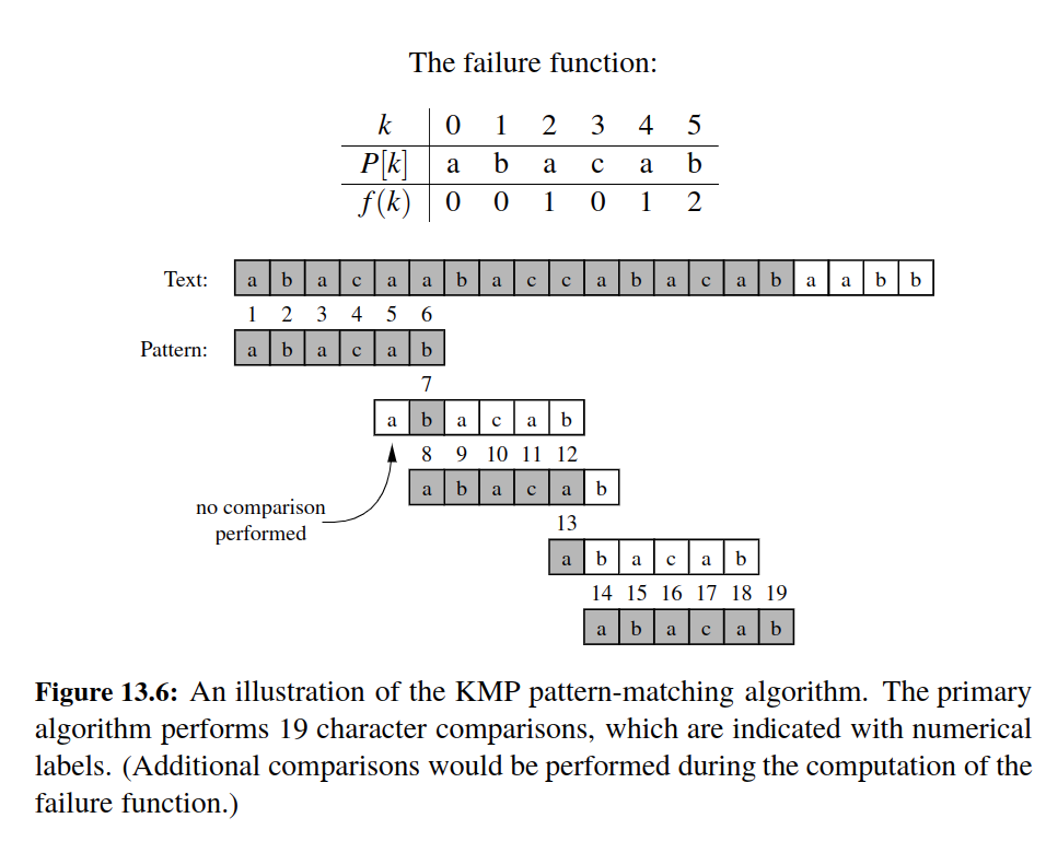
KMP - Knuth Morris Pratt¶

There is still a major inefficiency.

For a certain alignment of the pattern, if we find several matching characters but then detect a mismatch, we ignore all the information gained by the successful comparisons after restarting with the next incremental placement of the pattern.

The Knuth-Morris-Pratt (or “KMP”) algorithm, discussed in this section, avoids this waste of information and, in so doing, it achieves a running time of \(O(n+ m)\), which is asymptotically optimal.

The main idea of the KMP algorithm is to precompute self-overlaps between portions of the pattern so that when a mismatch occurs at one location, we immediately know the maximum amount to shift the pattern before continuing the search.

def find_kmp(T, P):
    """Return the lowest index of T at 
    which substring P begins (or else -1)."""
    n, m = len(T), len(P)  # introduce convenient notations
    if m == 0:
        return 0  # trivial search for an empty string
    fail = compute_kmp_fail(P)  # rely on utility to precompute
    j = 0  # index into text
    k = 0  # index into pattern
    while j < n:
        if T[j] == P[k]:  # P[0:1+k] matched thus far
            if k == m - 1:  # match is complete
                return j - m + 1
            j += 1  # try to extend match
            k += 1
        elif k > 0:
            k = fail[k - 1]  # reuse the suffix of P[0:k]
        else:
            j += 1
    return -1  # reached the end without a match

def compute_kmp_fail(P):
    """Utility that computes and returns KMP fail list."""
    m = len(P)
    fail = [0] * m  # by default, presume overlap of 0 everywhere
    j = 1
    k = 0
    while j < m:  # compute f(j) during this pass, if nonzero
        if P[j] == P[k]:  # k + 1 characters match thus far
            fail[j] = k + 1
            j += 1
            k += 1
        elif k > 0:  # k follows a matching prefix
            k = fail[k - 1]
        else:  # no match found starting at j
            j += 1
    return fail

find_kmp("alareference", "fer") # 5

The Knuth-Morris-Pratt algorithm performs pattern matching on a text string of length n and a pattern string of length m in \(O(n+ m)\) time.

Dynamic Programming¶

Dynamic programming can often be used to take problems that seem to require exponential time and produce polynomial-time algorithms to solve them.

In addition, the algorithms that result from applications of the dynamic programming technique are usually quite simple—often needing little more than a few lines of code to describe some nested loops for ﬁlling in a table.

Matrix Chain Product Example¶

Suppose we are given a collection of n two-dimensional matrices for which we wish to compute the mathematical product \(A = A_0 · A_1 · A_2 · · · A_{n−1}\) ,where \(A_i\) is a \(d_i × d_{i+1}\) matrix, for \(i = 0, 1, 2, . . . , n − 1\).

In the standard matrix multiplication algorithm (which is the one we will use), to multiply a d × e-matrix B times an e × f -matrix C, we compute the product, A, as

\[ A[i][ j] = \sum_{k=0}^{e-1} B[i][k] ·C[k][ j]. \]

This deﬁnition implies that matrix multiplication is associative, that is, it implies that \(B · (C · D) = (B · C) · D\).

Thus, we can parenthesize the expression for A anyway we wish and we will end up with the same answer.

However, we will not necessarily perform the same number of primitive (that is, scalar) multiplications in each parenthesization, as is illustrated in the following example.

Example

Let B be a 2 × 10-matrix, let C be a 10 × 50-matrix, and let D be a 50 × 20-matrix.

Computing B · (C · D) requires 2 · 10 · 20 + 10 · 50 · 20 = 10400 multiplications, whereas computing (B ·C) · D requires 2 · 10 · 50 + 2 · 50 · 20 = 3000 multiplications.

The matrix chain-product problem is to determine the parenthesization of the expression deﬁning the product A that minimizes the total number of scalar multiplications performed.

As the example above illustrates, the differences between parenthesizations can be dramatic, so ﬁnding a good solution can result in signiﬁcant speedups.

How ?

Define subproblems
Characterize Optimal Solutions

Here is a code example:

def matrix_chain(d):
    """d is a list of n+1 numbers such that size of kth matrix is d[k]-by-d[k+1].
    Return an n-by-n table such that N[i][j] represents the minimum number of
    multiplications needed to compute the product of Ai through Aj inclusive.
    """
    n = len(d) - 1                  # number of matrices
    N = [[0] * n for i in range(n)]   # initialize n-by-n result to zero
    for b in range(1, n):           # number of products in subchain
        for i in range(n-b):        # start of subchain
            j = i + b                   # end of subchain
            N[i][j] = min(N[i][k] + N[k+1][j] + d[i] * d[k+1] * d[j+1] for k in range(i,j))
    return N

dimensions = [10, 20, 30, 40, 30]
result = matrix_chain(dimensions)
print(result)

Let's break down how dynamic programming (DP) is used in the provided matrix_chain function and interpret the result:

Input: dimensions: A list representing the dimensions of matrices. The matrix A[i] has dimensions dimensions[i] x dimensions[i+1].
Output: The function returns a 2D table N, where N[i][j] represents the minimum number of scalar multiplications needed to compute the product of matrices A[i] through A[j] inclusively.
Dynamic Programming Approach: The function uses a bottom-up dynamic programming approach. It iteratively fills up the table N by considering different subchains of matrices and finding the optimal way to multiply them to minimize the number of scalar multiplications.
Table Filling: The outer loop (for b in range(1, n)) iterates over the number of matrices in the subchain. The inner loop (for i in range(n-b)) iterates over the starting matrix of the subchain. The variable j represents the end of the subchain. The inner loop then considers different partitions of the subchain by iterating over the variable k. For each partition, it calculates the cost of multiplying the matrices in that subchain and updates the table entry N[i][j] with the minimum cost.
Result Interpretation: The result, result, is the filled table N. Each entry N[i][j] contains the minimum number of scalar multiplications needed to compute the product of matrices from A[i] to A[j] inclusively in an optimal way.
Printing the Result: The print(result) statement outputs the filled table, showing the minimum number of scalar multiplications for each subchain of matrices.
Example: If dimensions = [10, 20, 30, 40, 30], the result will represent the minimum number of scalar multiplications for the optimal way to multiply matrices A[0] through A[4] inclusively.

[
 [0, 6000, 18000, 30000],
 [0, 0, 24000, 54000],
 [0, 0, 0, 36000],
 [0, 0, 0, 0]
]

For example, result[0][3] is 30000, indicating that the minimum number of scalar multiplications to compute the product of matrices A[0] through A[3] inclusively is 30000.

In summary, the result is a dynamic programming table that provides the optimal solution to the matrix chain multiplication problem, minimizing the number of scalar multiplications needed to compute the product of a sequence of matrices.

The dynamic programming approach avoids redundant calculations by solving and storing subproblems in a bottom-up fashion.

This was such a complex example. Here is a simpler one.

Fibonacci Series¶

Dynamic programming (DP) is a technique used in computer science and mathematics to solve optimization problems by breaking them down into simpler overlapping subproblems and solving each sub problem only once, storing the solutions to avoid redundant computations.

It is particularly useful when a problem has optimal substructure and overlapping subproblems.

Let's take the classic example of calculating the \(n_{th}\) Fibonacci number to illustrate dynamic programming.

The Fibonacci sequence is defined as follows:

\(F(n)=F(n−1)+F(n−2)\)

\(F(0)=0\) \(F(1)=1\)

Without dynamic programming, a straightforward recursive solution to calculate the \(n_{th}\) Fibonacci number might look like this in Python:

def fibonacci_recursive(n):
    if n <= 1:
        return n
    return fibonacci_recursive(n-1) + fibonacci_recursive(n-2)

Now, let's analyze the time complexity of this naive recursive solution. The time complexity is exponential, roughly \(O(2^n)\).

This is because for each Fibonacci number, the function makes two recursive calls, leading to an exponential number of calls.

Now, let's see how dynamic programming can significantly improve the efficiency of this solution.

DP Approach:¶

We can use memoization to store the results of previously solved subproblems and avoid redundant computations. Here's a simple dynamic programming solution using memoization in Python:

def fibonacci_dp(n, memo={}):
    if n <= 1:
        return n

    if n not in memo:
        memo[n] = fibonacci_dp(n-1, memo) + fibonacci_dp(n-2, memo)
    return memo[n]

In this solution, the memo dictionary is used to store the results of already computed Fibonacci numbers.

If a Fibonacci number is already in the memo, it is directly returned, preventing the need for redundant calculations.

Now, let's compare the two approaches for calculating \(F(5)\) using both the naive recursive approach and the dynamic programming approach.

The dynamic programming solution is much more efficient, especially for larger values of n. The time complexity of the dynamic programming solution is \(O(n)\) due to the memoization, making it exponentially faster than the naive recursive approach.

This example demonstrates the power of dynamic programming in optimizing solutions to problems with overlapping subproblems, and it is a fundamental technique in algorithm design.

The Components of a Dynamic Programming Solution¶

As mentioned above, the dynamic programming technique is used primarily for optimization problems, where we wish to ﬁnd the “best” way of doing something.

We can apply the dynamic programming technique in such situations if the problem has certain properties:

Simple Subproblems¶

There has to be some way of repeatedly breaking the global optimization problem into subproblems. Moreover, there should be a way to parameterize subproblems with just a few indices, like i, j, k, and so on.

Subproblem Optimization¶

An optimal solution to the global problem must be a composition of optimal subproblem solutions.

Subproblem Overlap¶

Optimal solutions to unrelated subproblems can contain subproblems in common.

Chat-GPT Wisdom¶

Dynamic programming is a technique for solving optimization problems by breaking them down into simpler overlapping subproblems and solving each subproblem only once, storing the solutions to subproblems to avoid redundant work.

This approach is especially useful when a problem has optimal substructure and overlapping subproblems.

Here's a breakdown of the key concepts and benefits of dynamic programming:

Optimal Substructure¶

This property means that an optimal solution to the problem contains optimal solutions to its subproblems.

In the matrix chain multiplication problem, the optimal way to multiply a sequence of matrices involves the optimal multiplication of its subsequences.

Overlapping Subproblems¶

Dynamic programming avoids redundant computation by solving subproblems only once and storing their solutions in a table or cache.

In the matrix chain multiplication problem, there are repeated calculations when considering different subsequences, which can be avoided using dynamic programming.

Memoization and Tabulation¶

Memoization involves storing the results of expensive function calls and returning the cached result when the same inputs occur again.

Tabulation involves filling a table with the results of subproblems and using those results to build up to the solution of the overall problem.

Benefits¶

Optimization: Dynamic programming often leads to more efficient solutions by avoiding redundant calculations.

Simplicity: It can simplify complex problems by breaking them down into smaller, manageable subproblems.

Readability: Dynamic programming solutions are often more readable and intuitive than alternative approaches.

Identifying Dynamic Programming Problems:¶

Optimal Substructure: If a problem can be broken down into smaller independent subproblems and the optimal solution to the problem can be constructed from optimal solutions to its subproblems, it may be suitable for dynamic programming.

Overlapping Subproblems: If the problem involves solving the same subproblems multiple times, dynamic programming can help by avoiding redundant computations.

Common Patterns for DP¶

Dynamic programming problems often exhibit one of two common patterns: bottom-up (tabulation) or top-down (memoization).

The matrix chain multiplication code you provided is an example of the bottom-up approach.

To identify when to use dynamic programming, consider whether the problem can be decomposed into overlapping subproblems with optimal substructure.

If these characteristics are present, dynamic programming might be a powerful approach to solving the problem.

Text Compression and Greedy Method¶

This part explains Greedy method from the lens of Huffman Coding.

Heads up: Given a string X defined over some alphabet, such as the ASCII or Unicode character sets, and we want to efficiently encode X into a small binary string Y (using only the characters 0 and 1).

Text compression is useful in any situation where we wish to reduce bandwidth for digital communications, so as to minimize the time needed to transmit our text.

Likewise, text compression is useful for storing large documents more efficiently, so as to allow a fixed-capacity storage device to contain as many documents as possible.

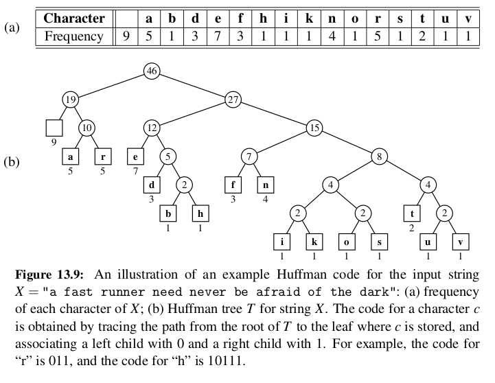
huffman_code_illustrated — Huffman Code Illustrated

Huffman Coding Algorithm¶

Huffman’s algorithm constructs an optimal prefix code for a string of length n with d distinct characters in O(n + d log d) time.

Greedy Method¶

This design pattern is applied to optimization problems, where we are trying to construct some structure while minimizing or maximizing some property of that structure.

We proceed by a sequence of choices.

The sequence starts from some well-understood starting condition, and computes the cost for that initial condition.

The pattern then asks that we iteratively make additional choices by identifying the decision that achieves the best cost improvement from all of the choices that are currently possible.

This approach does not always lead to an optimal solution.

But there are several problems that it does work for, and such problems are said to possess the greedy-choice property.

This is the property that a global optimal condition can be reached by a series of locally optimal choices (that is, choices that are each the current best from among the possibilities available at the time), starting from a well-deﬁned starting condition.

The problem of computing an optimal variable-length prefix code is just one example of a problem that possesses the greedy-choice property.

Tries¶

This approach is suitable for applications where a series of queries is performed on a fixed text, so that the initial cost of preprocessing the text is compensated by a speedup in each subsequent query (for example, a Web site that offers pattern matching in Shakespeare’s Hamlet or a search engine that offers Web pages on the Hamlet topic).

A trie (pronounced “try”) is a tree-based data structure for storing strings in order to support fast pattern matching. The main application for tries is in information retrieval.

Indeed, the name “trie” comes from the word “retrieval.”

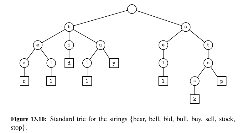
This is a standard Trie.

A standard trie storing a collection S of s strings of total length n from an alphabet Σ has the following properties:

The height of T is equal to the length of the longest string in S.
Every internal node of T has at most |Σ| children.
T has s leaves
The number of nodes of T is at most n + 1.

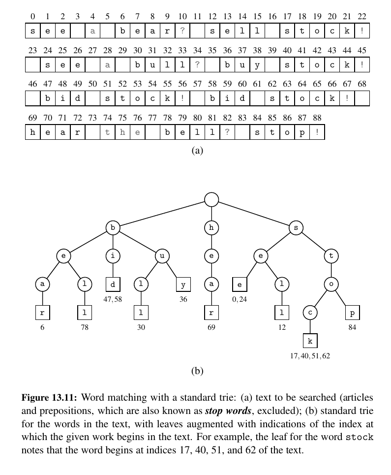
word_matching_with_trie — Word Matching with Trie

It is easy to see that the running time of the search for a string of length m is O(m · |Σ|), because we visit at most m + 1 nodes of T and we spend O(|Σ|) time at each node determining the child having the subsequent character as a label.

The O(|Σ|) upper bound on the time to locate a child with a given label is achievable, even if the children of a node are unordered, since there are at most |Σ| children.

We can improve the time spent at a node to be O(log |Σ|) or expected O(1), by mapping characters to children using a secondary search table or hash table at each node, or by using a direct lookup table of size |Σ| at each node, if |Σ| is sufﬁciently small (as is the case for DNA strings).

For these reasons, we typically expect a search for a string of length \(m\) to run in \(O(m)\) time.

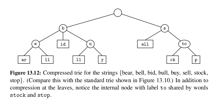
Compressed Tries¶

We can transform T into a compressed trie by replacing each redundant chain \((v_0 , v_1 ) · · · (v_{k−1} , v_k )\) of \(k ≥ 2\) edges into a single edge \((v_0 , v_k )\), relabeling \(v_k\) with the concatenation of the labels of nodes \(v_1 , . . . , v_k\) .

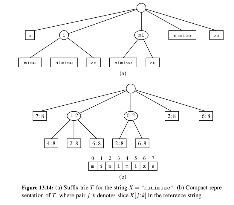
Suffix Tries¶

Using a sufﬁx trie allows us to save space over a standard trie by using several space compression techniques, including those used for the compressed trie.

Use cases:

Efficient Pattern Matching: One of the main applications of suffix tries is in pattern matching. Given a pattern, the trie allows for quick determination of whether the pattern exists in the original string.
Longest Common Substring: Suffix tries can be used to find the longest common substring between two or more strings efficiently.
Substring Retrieval: It allows for fast retrieval of all occurrences of a substring within the original string.

Almost there! Let's explore about Graphs now.