Sorting and Selection 🥰

Excited! 💕

Why Study Sorting Algorithms?

Why ?

• Many advanced algorithms for a variety of problems rely on sorting as a subroutine.

• Using Python, when calling the built in function, it is good to know what to expect in terms of efficient and how that may depend upon the initial order of elements or the type of objects that are being sorted.

• Ideas and approaches to sorting led to advances in the development in many other areas of computing.

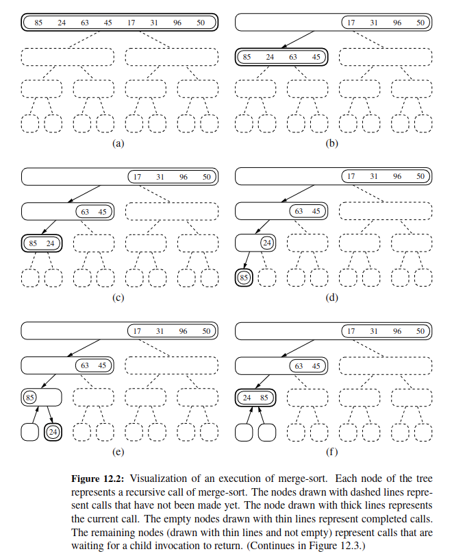
Merge Sort 🏋️‍♂️

It is using an algorithmic pattern called Divide and Conquer. This wonderful source explains how to approach divide and conquer.

If an algorithm exhibit overlapping sub problems, you can use divide and conquer.

Divide

If sequence has 0 or 1 element, return. If it has at least 2 elements, divide it into 2.

Conquer

Recursively sort sequences that you have as a result of dividing.

Combine

Put back sorted elements into S by merging the sorted sequences into one.

Here is the whole picture:

Merge Sort Execution

Here is step by step approach:

Merge Sort Visualized

Here is the code:

def merge_sort(seq):
    if len(seq) <= 1:
        return seq
    mid = len(seq) // 2
    # divide and conquer
    # recurring
    left = merge_sort(seq[:mid])
    right = merge_sort(seq[mid:])
    # combine
    return merge(left, right)

def merge(left, right):
    result = []
    i = j = 0
    while i < len(left) and j < len(right):
        if left[i] < right[j]:
            result.append(left[i])
            i += 1
        else:
            result.append(right[j])
            j += 1
    # why do we do this ?
    result.extend(left[i:])
    result.extend(right[j:])
    return result

array = [38, 27, 43, 3, 9, 82]
print("Sorted Array:", merge_sort(array)) # Sorted Array: [3, 9, 27, 38, 43, 82]

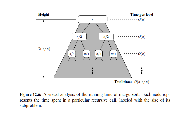
Running time of MergeSort

Answer: o(n(log(n))

Merge method : \(O(n_1+ n_2)\) - The merge function iterates through both left and right arrays exactly once, which takes \(O(n)\) time in total, where \(n\) is the combined length of left and right.

Merge Sort Method: \(log(n)\) is the height of the tree, for each division we get that. To divide every node on a tree for merge sort will be proportional to \(log(n)\) time and we have \(o(n)\) time complexity for n elements in seq.

Running time of Merge Sort

Just a heads up, you can also use a recurrence relation here.

You can also implement merge sort without recursion.

Here is the code for non recursive version:

import math

def merge(src, result, start, inc):
    """Merge src[start:start+inc] and src[start+inc:start+2*inc] into result."""
    end1 = start + inc  # boundary for run 1
    end2 = min(start + 2 * inc, len(src))  # boundary for run 2
    x, y, z = start, start + inc, start  # index into run 1, run 2, result
    while x < end1 and y < end2:
        if src[x] < src[y]:
            result[z] = src[x]
            x += 1
        else:
            result[z] = src[y]
            y += 1
        z += 1  # increment z to reflect new result
    if x < end1:
        result[z:end2] = src[x:end1]  # copy remainder of run 1 to output
    elif y < end2:
        result[z:end2] = src[y:end2]  # copy remainder of run 2 to output


def merge_sort(S):
    """Sort the elements of Python list S using the merge-sort algorithm."""
    n = len(S)
    logn = math.ceil(math.log(n, 2))
    src, dest = S, [None] * n  # make temporary storage for dest
    for i in (2 ** k for k in range(logn)):  # pass i creates all runs of length 2i
        for j in range(0, n, 2 * i):  # each pass merges two length i runs
            merge(src, dest, j, i)
        src, dest = dest, src  # reverse roles of lists
    if S is not src:
        S[0:n] = src[0:n]  # additional copy to get results to S

a = [51234,43,1234,51,234,51,2,3,57,9,4,1]
merge_sort(a)
print(a) # [1, 2, 3, 4, 9, 43, 51, 51, 57, 234, 1234, 51234]

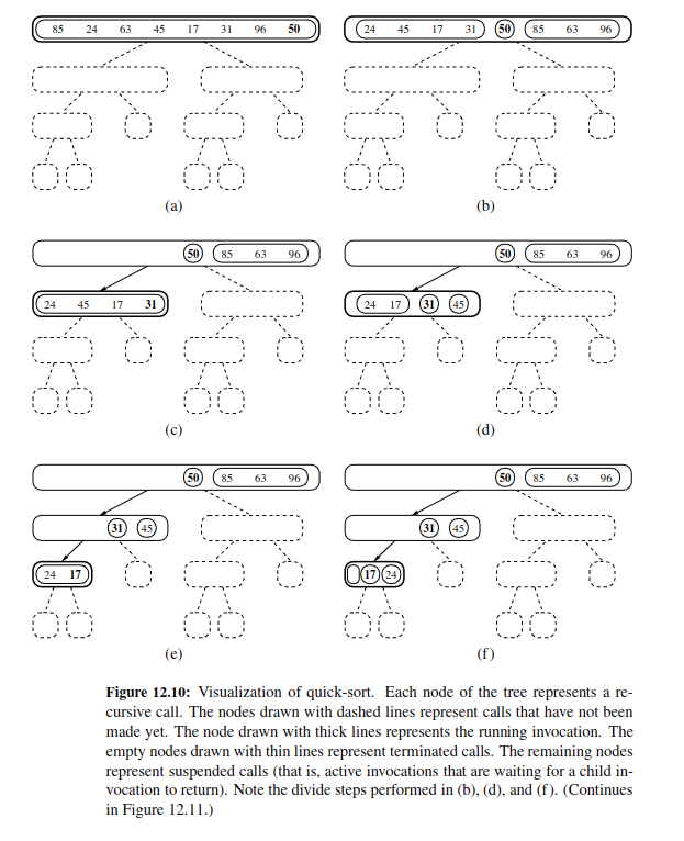
Quick Sort 🧠

Quick sort is also based on Divide and Conquer algorithm. The key thing is the pivot.

Divide

If S has at least two elements (nothing needs to be done if S has zero or one element), select a specific element x from S, which is called the pivot.

As is common practice, choose the pivot x to be the last element in S.

Remove all the elements from S and put them into three sequences:

• L, storing the elements in S less than x

• E, storing the elements in S equal to x

• G, storing the elements in S greater than x

Of course, if the elements of S are distinct, then E holds just one element - the pivot itself.

Conquer

Recursively sort sequences L and G.

Combine

Put back the elements into S in order by first inserting the elements of L, then those of E, and finally those of G.

Visualize Quick Sort

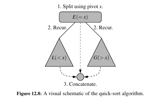
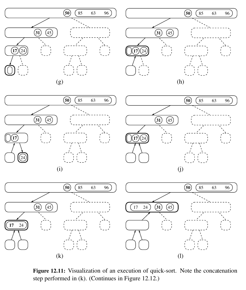
Here it how it works in single figure:

Quick Sort Execution

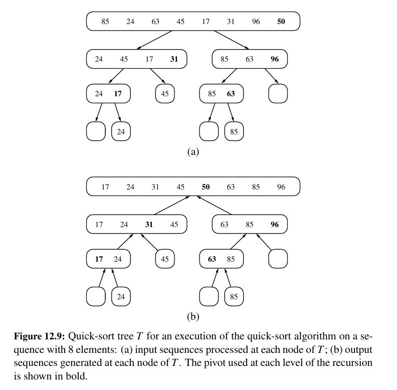
Here is how it works step by step:

Initial Steps of Quick Sort

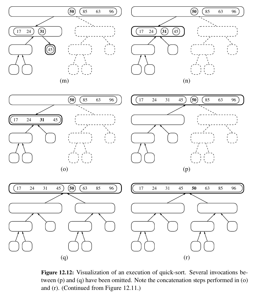
After all the left side is done, we move on to the right side.

Quick Sort Continued

And the ending.

Quick Sort Ending

Running time of Quick Sort

Worst case \(o(n^2)\).

The height of the tree on quick sort is worst case \(o(n - 1)\) NOT \(o(logn)\) like it was on merge sort.

This is because the splitting while comparing to pivot is not guaranteed to be half-half.

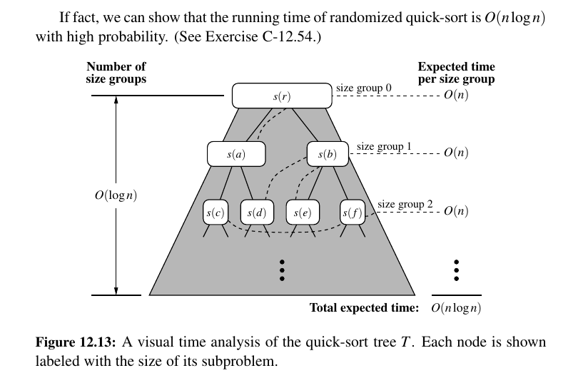
Randomized Quick Sort

There is randomized quick sort where we select the pivot randomly from the sequence.

The expected running time of randomized quick-sort on a sequence S of size \(n\) is \(O(n log n)\).

Visual Running Time of Quick Sort

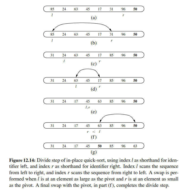
In Place Quick Sort

An algorithm is in-place if it uses only a small amount of memory in addition to that needed for the original input.

Our implementation of heap-sort, from Chapter 9.4.2, is an example of such an in-place sorting algorithm.

Quick-sort of an array-based sequence can be adapted to be in-place, and such an optimization is used in most deployed implementations.

In place Quick Sort:

def inplace_quick_sort(S, a, b):
    """Sort the list from S[a] to S[b] inclusive using the quick-sort algorithm."""
    if a >= b: return # range is trivially sorted
    pivot = S[b] # last element of range is pivot
    left = a # will scan rightward
    right = b-1 # will scan leftward
    while left <= right: 
        # scan until reaching value equal or larger than pivot (or right marker)
        while left <= right and S[left] < pivot:
            left += 1
        # scan until reaching value equal or smaller than pivot (or left marker)
        while left <= right and pivot < S[right]:
            right -= 1 
        if left <= right: # scans did not strictly cross
            S[left], S[right] = S[right], S[left] # swap values 
            left, right = left + 1, right - 1 # shrink range
    # put pivot into its final place (currently marked by left index)
    S[left], S[b] = S[b], S[left]
    # make recursive calls
    inplace_quick_sort(S, a, left - 1)
    inplace_quick_sort(S, left + 1, b)


seq = [2,4,5,621,324,123,45324]
inplace_quick_sort(seq, 0, len(seq)-1)
print(seq) # [2, 4, 123, 324, 621, 45324]

The main idea behind quick sort is that, we select a pivot, we select two pointers that we are interested in.

We keep comparing the values in those pointers and swap when needed.

At last, put the pivot just before the right pointer as it should be there.

Divide for in place Quick Sort

Just a heads up: There is also another method for selecting the pivot, median of three.

Tip

Quick sort has very good performance on large datasets, it is not good for small datasets.

In small datasets, insertion sort might be just way faster.

It is therefore common, in optimized sorting implementations, to use a hybrid approach, with a divide-and-conquer algorithm used until the size of a subsequence falls below some threshold (perhaps 50 elements); insertion-sort can be directly invoked upon portions with length below the threshold.

Sorting - Through an Algorithmic Sense

The best we can do is \(O(n log n)\) in the worst case. No getting around it. Because this is a comparison based sort.

Linear Time Sorting on Special Assumptions

Can there be anything faster than \(O(n(log(n)))\) ? Under some conditions, yeah.

Bucket Sort

Consider a sequence S of n entries whose keys are integers in the range [0, N −1], for some integer \(N ≥2\), and suppose that S should be sorted according to the keys of the entries.

In this case, it is possible to sort S in \(O(n+ N)\) time.

It might seem surprising, but this implies, for example, that if N is \(O(n)\), then we can sort S in \(O(n)\) time.

def bucket_sort(seq):
    # Find the minimum and maximum values in the sequence
    min_val = min(seq) # o(n)
    max_val = max(seq) # o(n)

    # Create a list of buckets, one for each possible value
    buckets = [0] * (max_val - min_val + 1)

    # Place elements in their respective buckets
    for num in seq:
        buckets[num - min_val] += 1

    # Reconstruct the sorted sequence from the buckets
    sorted_seq = []
    for i, count in enumerate(buckets):
        sorted_seq.extend([i + min_val] * count)

    return sorted_seq

seq = [1, 2, 5, 6, 7, 4, 9, 3]
sorted_seq = bucket_sort(seq)
print("Sorted Sequence:", sorted_seq)
# Sorted Sequence: [1, 2, 3, 4, 5, 6, 7, 9]

Bucket sort is most effective when the range(k) is not significantly larger than the number of elements \((n)\) in the input sequence.

This is because the range of values determines the number of buckets created, and if the range is much larger than the number of elements, it can lead to the creation of many empty buckets.

In such cases, the algorithm's efficiency decreases, and it may not provide a significant advantage over other sorting algorithms with a time complexity of \(O(n * log n)\), like quick-sort or merge-sort.

In summary, the effectiveness of bucket sort is contingent on having a reasonably uniform distribution of values within the range, and it's well-suited for situations where the range is not excessively larger than the number of elements.

Stable Sorting

When sorting key-value pairs, an important issue is how equal keys are handled.

Let \(S = (( k_0, v_0), . . . , (k_{n−1} , v_{n−1}))\) be a sequence of such entries.

We say that a sorting algorithm is stable if, for any two entries \((k_i, v_i)\) and \((k_j, v_j)\) of S such that \(k_i = k_j\) and \((k_i, v_i)\) precedes \((k_j, v_j)\) in S before sorting (that is, i < j), entry \((k_i, v_i)\) also precedes entry \((k_j, v_j)\) after sorting.

Stability is important for a sorting algorithm because applications may want to preserve the initial order of elements with the same key.

Radix Sort 🤨

The radix-sort algorithm sorts a sequence S of entries with keys that are pairs, by applying a stable bucket-sort on the sequence twice; first using one component of the pair as the key when ordering and then using the second component

Allegedly, here is an example of Radix sort.

def counting_sort(arr, exp):
    n = len(arr)
    output = [0] * n
    count = [0] * 10  # Make a count list to store the count of each digit (0-9).
    # Count the occurrences of each digit based on the current digit place.
    for i in range(n):
        index = arr[i] // exp
        count[index % 10] += 1

    # Modify the count array to store the actual position of each digit.
    for i in range(1, 10):
        count[i] += count[i - 1]

    # Build the output array by placing elements in the correct order.
    i = n - 1
    while i >= 0:
        index = arr[i] // exp
        output[count[index % 10] - 1] = arr[i]
        count[index % 10] -= 1
        i -= 1

    # Copy the sorted elements from the output array back to the original array.
    for i in range(n):
        arr[i] = output[i]

def radix_sort(arr):
    max_value = max(arr)  # Find the maximum value in the array.
    exp = 1  # Initialize the digit place to the least significant digit.

    # Iterate through each digit place, from the least significant to most.
    while max_value // exp > 0:
        # Sort the array based on the current digit place.
        counting_sort(arr, exp)
        exp *= 10  # Move to the next digit place.

# Example usage:
arr = [170, 45, 75, 90, 802, 24, 2, 66]
radix_sort(arr)
print("Sorted array:", arr)
# Sorted array: [2, 24, 45, 66, 75, 90, 170, 802]

Comparing Sorting Algorithms

Tip

While selecting a sorting algorithm, there are trade offs involving efficiency, memory usage and stability.

Tradeoffs

The tradeoffs are around efficiency, memory usage and stability.

Insertion Sort

For sorting small sequences, this is great. Also great for almost sorted stuff.

That means number of inversions is small. Running time for these is \(O(n + m)\) , where m is the number of inversions.

Heap Sort

\(O(n log n)\) worst case. On larger sequences, quick sort and merge sort outperforms it. It is not stable.

Quick Sort

Not stable.

It can outperform heap sort and merge sort. It was the default choice in C and Java through version 6.

1. Cache Efficiency: Quicksort often exhibits better cache performance. In quicksort, the partitioning process involves swapping elements based on a pivot, which are usually located in adjacent memory locations. This behavior can lead to better cache utilization, as elements being processed are likely to be in close proximity in memory. In contrast, heap sort and merge sort involve more random access to memory, which can result in cache misses and slower performance.

2. In-Place Sorting: Quicksort can be implemented in an in-place manner, which means it doesn't require additional memory for auxiliary data structures. In contrast, merge sort typically requires extra memory for merging two subarrays, and heap sort requires a separate heap data structure. In situations where memory usage is a concern, quicksort may be a more attractive choice.

3. Average-Case Efficiency: Quicksort's expected average-case time complexity is \(O(n log n)\), which is efficient. It performs well on average for random or well-distributed data, making it suitable for a wide range of real-world datasets.

4. Fewer Comparisons: Quicksort often requires fewer comparisons and swaps than merge sort, making it more efficient for smaller datasets. This can be an advantage when sorting small or moderately sized lists.

Merge Sort

Merge-sort runs in \(O(n log n)\) time in the worst case.

It is quite difficult to make merge-sort run in-place for arrays, and without that optimization the extra overhead of allocate a temporary array, and copying between the arrays is less attractive than in-place implementations of heap-sort and quick-sort for sequences that can fit entirely in a computer’s main memory.

The GNU sorting utility (and most current versions of the Linux operating system) relies on a multiway merge-sort variant.

Tip

Here is some wisdom.

Since 2003, the standard sort method of Python’s list class has been a hybrid approach named Tim-sort (designed by Tim Peters), which is essentially a bottom-up merge-sort that takes advantage of some initial runs in the data while using insertion-sort to build additional runs.

You can read about TimSort from Tim in this link in the codebase

Tim-sort has also become the default algorithm for sorting arrays in Java7.

Name	Best	Average	Worst	Memory	Stable	Method	Other notes
Heapsort	n log (n)	n log (n)	n log (n)	Selection	No
Merge sort	n log (n)	n log (n)	n log (n)	n	Yes	Merging	Highly parallelizable (up to O(log n) using the Three Hungarians' Algorithm).
Timsort	n	n log (n)	n log (n)	n	Yes	Insertion & Merging	Makes n-1 comparisons when the data is already sorted or reverse sorted.
Quicksort	n log (n)	n log (n)	n ^ 2	log (n)	No	Partitioning	Quicksort is usually done in-place with O(log n) stack space.
Insertion sort	n	n ^ 2	n ^ 2	1	Yes	Insertion	O(n + d), in the worst case over sequences that have d inversions.
Bubble sort	n	n ^ 2	n ^ 2	1	Yes	Exchanging	Tiny code size.
Selection sort	n ^ 2	n ^ 2	n ^ 2	1	No	Selection	Stable with O(n) extra space, when using linked lists, or when made as a variant of Insertion Sort instead of swapping the two items.
Cycle sort	n ^ 2	n ^ 2	n ^ 2	1	No	Selection	In-place with theoretically optimal number of writes.

2 More Sorts - Just because we are curious.

Smooth Sort

An adaptive variant of heapsort based upon the Leonardo sequence rather than a traditional binary heap.

In computer science, smoothsort is a comparison-based sorting algorithm.

A variant of heapsort, it was invented and published by Edsger Dijkstra in 1981. Like heapsort, smoothsort is an in-place algorithm with an upper bound of O(n log n) operations  but it is not a stable sort.

The advantage of smoothsort is that it comes closer to O(n) time if the [input is already sorted to some degree], whereas heapsort averages O(n log n ) regardless of the initial sorted state.

Advantages

• Smooth Sort is an adaptive sorting algorithm, meaning that it performs well on partially sorted lists.

• The algorithm has a time complexity of O(n log n), which is the same as merge sort and heap sort.

• Smooth Sort uses a small amount of extra memory and has a low memory overhead compared to other sorting algorithms, such as merge sort.

Disadvantages

• Smooth Sort is a complex algorithm, and it is more difficult to implement than some other sorting algorithms, such as insertion sort.

• The algorithm requires the use of Leonardo numbers, which are a less well-known mathematical concept, so the algorithm may not be as widely used or understood as other algorithms.

Allegedly, here is the code:

def smooth_sort(arr):
    n = len(arr)

    # Define the Leonardo numbers
    def leonardo(k):
        if k < 2:
            return 1
        return leonardo(k - 1) + leonardo(k - 2) + 1

    # Build the Leonardo heap by merging
    # pairs of adjacent trees
    def heapify(start, end):
        i = start
        j = 0
        k = 0

        while k < end - start + 1:
            if k & 0xAAAAAAAA:
                j = j + i
                i = i >> 1
            else:
                i = i + j
                j = j >> 1

            k = k + 1

        while i > 0:
            j = j >> 1
            k = i + j
            while k < end:
                if arr[k] > arr[k - i]:
                    break
                arr[k], arr[k - i] = arr[k - i], arr[k]
                k = k + i

            i = j

    # Build the Leonardo heap by merging
    # pairs of adjacent trees
    p = n - 1
    q = p
    r = 0
    while p > 0:
        if (r & 0x03) == 0:
            heapify(r, q)

        if leonardo(r) == p:
            r = r + 1
        else:
            r = r - 1
            q = q - leonardo(r)
            heapify(r, q)
            q = r - 1
            r = r + 1

        arr[0], arr[p] = arr[p], arr[0]
        p = p - 1

    # Convert the Leonardo heap
    # back into an array
    for i in range(n - 1):
        j = i + 1
        while j > 0 and arr[j] < arr[j - 1]:
            arr[j], arr[j - 1] = arr[j - 1], arr[j]
            j = j - 1

    return arr


# Driver ccode
arr = [1, 7, 8, 2, 3, 5, 4, 6]

# Original Array
print('Input: ', arr) # Input: [1, 7, 8, 2, 3, 5, 4, 6]

# Function call
print("Output: ", smooth_sort(arr)) # Output: [1, 2, 3, 4, 5, 6, 7, 8]

Block Sort

Block sort, or block merge sort, is a sorting algorithm combining at least two merge operations with an insertion sort to arrive at O(n log n) (see Big O notation) in-place stable sorting time.

It gets its name from the observation that merging two sorted lists, A and B, is equivalent to breaking A into evenly sized blocks, inserting each A block into B under special rules, and merging AB pairs.

Pythons Built in Sorting

Let's see some code to discover!

seq = [5,7,4,23]
seq.sort() # no new object, the seq is sorted

sorted(seq) # makes a new list object

We can use a key to sort sequences with the built in method. This works with decorate-sort-undecorate pattern.

![[fig12.16.png]]

colors = ["cyan", "white", "black", "magenta", "red"]
print(sorted(colors, key = len)) 
# ['red', 'cyan', 'white', 'black', 'magenta']

my_tuples_in_town = [(9,2), (6,3), (3,4), (0,5)]
print("Sorted based on first element:", sorted(my_tuples_in_town, key = lambda x : x[0]))
# Sorted based on first element: [(0, 5), (3, 4), (6, 3), (9, 2)]

my_dict = { 4: "asdf", 2: "asdz", 0: "seq"}
print(sorted(my_dict, key = my_dict.get)) # # [4, 2, 0]

# For example, here’s a case-insensitive string comparison:
sorted("This is a test string from Andrew".split(), key=str.lower)
# ['a', 'Andrew', 'from', 'is', 'string', 'test', 'This']

Selection

As important as it is, sorting is not the only interesting problem dealing with a total order relation on a set of elements.

There are a number of applications in which we are interested in identifying a single element in terms of its rank relative to the sorted order of the entire set.

Examples include identifying the minimum and maximum elements, but we may also be interested in, say, identifying the median element, that is, the element such that half of the other elements are smaller and the remaining half are larger.

In general, queries that ask for an element with a given rank are called order statistics.

Finding the \(kth\) smallest element - kthsmallest

This method below runs expected \(O(n)\) but worst case \(O(n^2)\)

import random

def quick_select(S, k):
    """Return the kth smallest element of list S, for k from 1 to len(S)."""
    if len(S) == 1:
        return S[0]
    pivot = random.choice(S) # pick random pivot element from S
    L = [x for x in S if x < pivot] # elements less than pivot
    E = [x for x in S if x == pivot] # elements equal to pivot
    G = [x for x in S if pivot < x] # elements greater than pivot
    if k <= len(L):
        return quick_select(L, k) # kth smallest lies in L
    elif k <= len(L) + len(E): 
        return pivot # kth smallest equal to pivot
    else:
        j = k - len(L) - len(E) # new selection parameter
        return quick_select(G, j) # kth smallest is jth in G

quick_select([1,23,45,1234,2,5], 2)

Marvelous! Let's discover text processing now!