Priority Queues

The Priority Queue Abstract Data Type

Priorities ✏️

In this chapter, we introduce a new abstract data type known as a priority queue.

This is a collection of prioritized elements that allows arbitrary element insertion, and allows the removal of the element that has first priority.

When an element is added to a priority queue, the user designates its priority by providing an associated key.

The element with the minimum key will be the next to be removed from the queue (thus, an element with key 1 will be given priority over an element with key 2).

Although it is quite common for priorities to be expressed numerically, any Python object may be used as a key, as long as the object type supports a consistent meaning for the test a < b, for any instances a and b, so as to define a natural order of the keys.

With such generality, applications may develop their own notion of priority for each element.

For example, different financial analysts may assign different ratings (i.e., priorities) to a particular asset, such as a share of stock.

The Priority Queue ADT

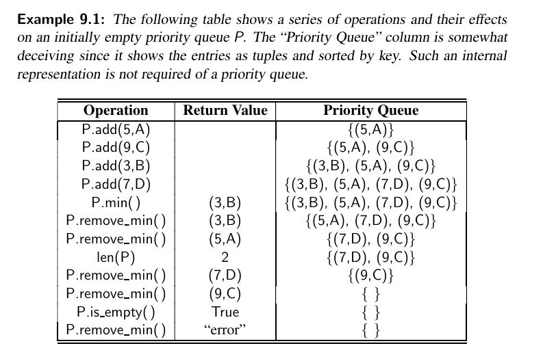
Formally, we model an element and its priority as a key-value pair. We define the priority queue ADT to support the following methods for a priority queue P:

P.add(k, v): Insert an item with key k and value v into priority queue P.

P.min(): Return a tuple, (k,v), representing the key and value of an item in priority queue P with minimum key (but do not remove the item); an error occurs if the priority queue is empty.

P.remove_min(): Remove an item with minimum key from priority queue P, and return a tuple, (k,v), representing the key and value of the removed item; an error occurs if the priority queue is empty.

P.is_empty(): Return True if priority queue P does not contain any items.

len(P): Return the number of items in priority queue P.

A priority queue may have multiple entries with equivalent keys, in which case methods min and remove_min may report an arbitrary choice of item having minimum key. Values may be any type of object.

Here is an example:

Priority Queue Methods

Extra - Priority Queues in Real World 🥰

Python implements priority queues with heaps. A min heap is all you need!

from heapq import heapify, heappop, heappush

a = [4,2,1,6,5,8,2]
# O(n)
heapify(a)

print(a) # [1, 2, 2, 6, 5, 8, 4]

# O(log(n))
print(heappop(a)) # 1
print(a) # [2, 2, 4, 6, 5, 8]

# O(log(n))
print(heappop(a)) # 2
print(a) # [2, 5, 4, 6, 8]

# heaps adjust lists in place
print(a[0] == 2) # True
print(a[1] == 5) # True
print(a[2] == 4) # True
print(a[3] == 6) # True
print(a[4] == 8) # True

Implementing a Priority Queue

In this section, we show how to implement a priority queue by storing its entries in a positional list L.

The Composition Design Pattern

...

TODO: Not urgent

...

The code:

class PriorityQueueBase:
    """Abstract base class for a priority queue."""

    # ------------------------------ nested _Item class ------------------------------
    class _Item:
        """Lightweight composite to store priority queue items."""
        __slots__ = '_key', '_value'

        def __init__(self, k, v):
            self._key = k
            self._value = v

        def __lt__(self, other):
            return self._key < other._key  # compare items based on their keys

        def __repr__(self):
            return '({0},{1})'.format(self._key, self._value)

    # ------------------------------ public behaviors ------------------------------
    def is_empty(self):  # concrete method assuming abstract len
        """Return True if the priority queue is empty."""
        return len(self) == 0

    def __len__(self):
        """Return the number of items in the priority queue."""
        raise NotImplementedError('must be implemented by subclass')

    def add(self, key, value):
        """Add a key-value pair."""
        raise NotImplementedError('must be implemented by subclass')

    def min(self):
        """Return but do not remove (k,v) tuple with minimum key.
        Raise Empty exception if empty.
        """
        raise NotImplementedError('must be implemented by subclass')

    def remove_min(self):
        """Remove and return (k,v) tuple with minimum key.
        Raise Empty exception if empty.
        """
        raise NotImplementedError('must be implemented by subclass')

Implementation with an Unsorted List

TODO: Not urgent

...

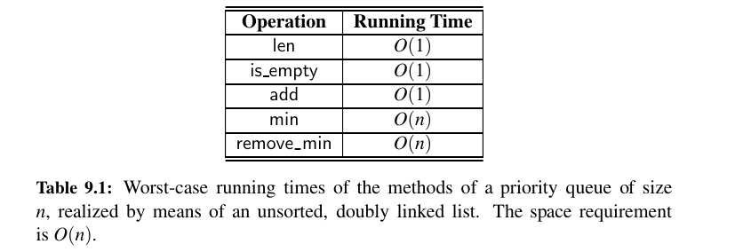
Worst case running times as follows:

Worst Case Running Times of Priority Queue

The code:

class UnsortedPriorityQueue(PriorityQueueBase):  # base class defines _Item
    """A min-oriented priority queue implemented with an unsorted list."""

    # ----------------------------- nonpublic behavior -----------------------------
    def _find_min(self):
        """Return Position of item with minimum key."""
        if self.is_empty():  # is_empty inherited from base class
            raise Empty('Priority queue is empty')
        small = self._data.first()
        walk = self._data.after(small)
        while walk is not None:
            if walk.element() < small.element():
                small = walk
            walk = self._data.after(walk)
        return small

    # ------------------------------ public behaviors ------------------------------
    def __init__(self):
        """Create a new empty Priority Queue."""
        self._data = PositionalList()

    def __len__(self):
        """Return the number of items in the priority queue."""
        return len(self._data)

    def add(self, key, value):
        """Add a key-value pair."""
        self._data.add_last(self._Item(key, value))

    def min(self):
        """Return but do not remove (k,v) tuple with minimum key.
        Raise Empty exception if empty.
        """
        p = self._find_min()
        item = p.element()
        return (item._key, item._value)

    def remove_min(self):
        """Remove and return (k,v) tuple with minimum key.
        Raise Empty exception if empty.
        """
        p = self._find_min()
        item = self._data.delete(p)
        return (item._key, item._value)

Implementation with a Sorted List

TODO: Not urgent

...

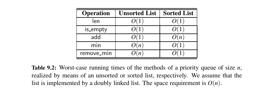
Worst case running times - comparison with unsorted:

Worst Case Running Times of Priority Queue - with a Sorted List

The Code:

class SortedPriorityQueue(PriorityQueueBase):  # base class defines _Item
    """A min-oriented priority queue implemented with a sorted list."""

    # ------------------------------ public behaviors ------------------------------
    def __init__(self):
        """Create a new empty Priority Queue."""
        self._data = PositionalList()

    def __len__(self):
        """Return the number of items in the priority queue."""
        return len(self._data)

    def add(self, key, value):
        """Add a key-value pair."""
        newest = self._Item(key, value)  # make new item instance
        walk = self._data.last()  # walk backward looking for smaller key
        while walk is not None and newest < walk.element():
            walk = self._data.before(walk)
        if walk is None:
            self._data.add_first(newest)  # new key is smallest
        else:
            self._data.add_after(walk, newest)  # newest goes after walk

    def min(self):
        """Return but do not remove (k,v) tuple with minimum key.
        Raise Empty exception if empty.
        """
        if self.is_empty():
            raise Empty('Priority queue is empty.')
        p = self._data.first()
        item = p.element()
        return (item._key, item._value)

    def remove_min(self):
        """Remove and return (k,v) tuple with minimum key.
        Raise Empty exception if empty.
        """
        if self.is_empty():
            raise Empty('Priority queue is empty.')
        item = self._data.delete(self._data.first())
        return (item._key, item._value)

Heaps 💯

The two strategies for implementing a priority queue ADT in the previous section demonstrate an interesting trade-off.

When using an unsorted list to store entries, we can perform insertions in \(O(1)\) time, but finding or removing an element with minimum key requires an \(O(n)\)-time loop through the entire collection.

What are Heaps?

In contrast, if using a sorted list, we can trivially find or remove the minimum element in \(O(1)\) time, but adding a new element to the queue may require \(O(n)\) time to restore the sorted order.

We provide a more efficient realization of a priority queue using a data structure called a binary heap.

This data structure allows us to perform both insertions and removals in logarithmic time, which is a significant improvement over the list-based implementations discussed in Section 9.2.

The fundamental way the heap achieves this improvement is to use the structure of a binary tree to find a compromise between elements being entirely unsorted and perfectly sorted.

If you want to understand heaps just check this wonderful tool.

A min heap has the smallest elements close to the root. 😉

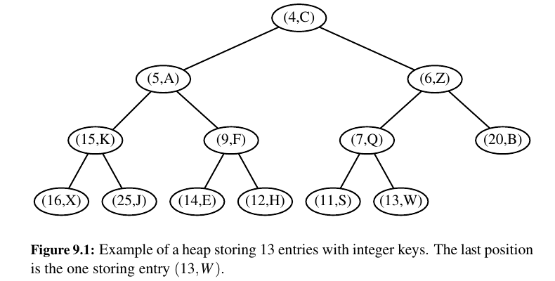
The Heap Data Structure 💖

Heap-Order Property: In a heap T , for every position p other than the root, the key stored at p is greater than or equal to the key stored at p’s parent.

Complete Binary Tree Property: A heap T with height h is a complete binary tree if levels \(0, 1, 2, . . . , h − 1\) of T have the maximum number of nodes possible (namely, level \(i\) has \(2i\) nodes, for \(0 ≤ i ≤ h − 1\)) and the remaining nodes at level h reside in the leftmost possible positions at that level.

Heap example

The Height of a Heap

Let h denote the height of T . Insisting that T be complete also has an important consequence, as shown in Proposition 9.2.

Proposition 9.2: A heap T storing n entries has height \(h = ⌊log(n)⌋\) (\(h = ⌊log(n)⌋\) - floor of log n).

Implementing a Priority Queue with a Heap

Adding an Item to the Heap

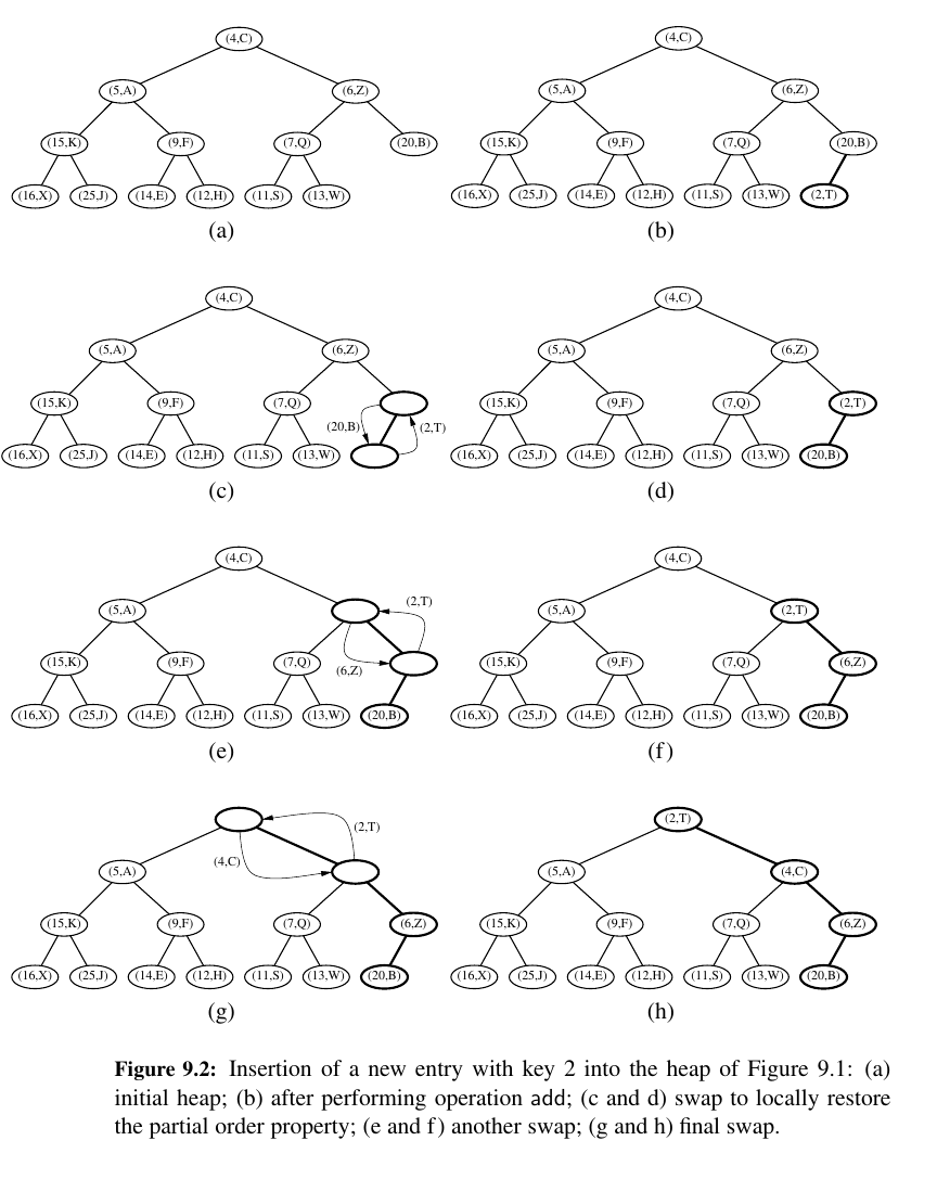
Let us consider how to perform add(k,v) on a priority queue implemented with a heap T.

We store the pair (k, v) as an item at a new node of the tree.

To maintain the complete binary tree property, that new node should be placed at a position p just beyond the rightmost node at the bottom level of the tree, or as the leftmost position of a new level, if the bottom level is already full (or if the heap is empty).

Up-Heap Bubbling After an Insertion

After this action, the tree T is complete, but it may violate the heap-order property.

The upward movement of the newly inserted entry by means of swaps is conventionally called up-heap bubbling.

A swap either resolves the violation of the heap-order property or propagates it one level up in the heap. In the worst case, up-heap bubbling causes the new entry to move all the way up to the root of heap T.

Thus, in the worst case, the number of swaps performed in the execution of method add is equal to the height of T . That bound is \(⌊(log(n))⌋\)

Heap swaps with Insertion!

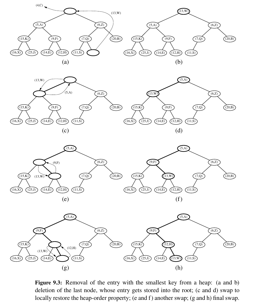
Removing the Item with Minimum Key

Let us now turn to method remove_min of the priority queue ADT. We know that an entry with the smallest key is stored at the root r of T (even if there is more than one entry with smallest key).

However, in general we cannot simply delete node r, because this would leave two disconnected subtrees. 🤭

Instead, we ensure that the shape of the heap respects the complete binary tree property by deleting the leaf at the last position p of T, defined as the rightmost position at the bottom most level of the tree.

Down-Heap Bubbling After a Removal

We are not yet done, however, for even though T is now complete, it likely violates the heap-order property.

Having restored the heap-order property for node p relative to its children, there may be a violation of this property at c; hence, we may have to continue swapping down T until no violation of the heap-order property occurs (See Figure 9.3.).

This downward swapping process is called down-heap bubbling. A swap either resolves the violation of the heap-order property or propagates it one level down in the heap.

In the worst case, an entry moves all the way down to the bottom level (see Figure 9.3).

Thus, the number of swaps performed in the execution of method remove min is, in the worst case, equal to the height of heap T, that is, it is \(⌊(log(n))⌋\).

Removing Smallest from Heap

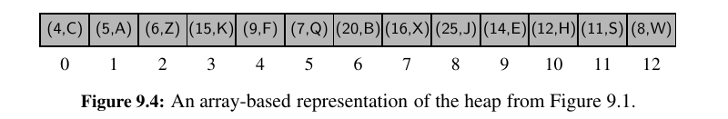
Array-Based Representation of a Complete Binary Tree

The array-based representation of a binary tree (Section 8.3.2) is especially suitable for a complete binary tree T.

We recall that in this implementation, the elements of T are stored in an array-based list such that the element at position p in T is stored in A with index equal to the level number \(f(p)\) of \(p\), defined as follows:

• If p is the root of T , then \(f (p) = 0\).

• If p is the left child of position q, then \(f (p) = 2 f (q) + 1\).

• If p is the right child of position q, then \(f (p) = 2 f (q) + 2\).

With this implementation, the elements of T have contiguous indices in the range [0, n − 1] and the last position of T is always at index \(n − 1\), where n is the number of positions of T.

Array Based Representation of Heaps

Implementing a priority queue using an array-based heap representation allows us to avoid some complexities of a node-based tree structure.

In particular, the add and remove_min operations of a priority queue both depend on locating the last index of a heap of size n.

With the array-based representation, the last position is at index \(n − 1\) of the array. Locating the last position of a complete binary tree implemented with a linked structure requires more effort. (See Exercise C-9.34.)

If the size of a priority queue is not known in advance, use of an array-based representation does introduce the need to dynamically resize the array on occasion, as is done with a Python list.

The space usage of such an array-based representation of a complete binary tree with n nodes is \(O(n)\), and the time bounds of methods for adding or removing elements become amortized. (See Chapter 5.3.1.)

Python Heap Implementation

We use an array-based representation, maintaining a Python list of item composites.

Here is the code:

class HeapPriorityQueue(PriorityQueueBase):  # base class defines _Item
    """A min-oriented priority queue implemented with a binary heap."""

    # ------------------------------ nonpublic behaviors ------------------------------
    def _parent(self, j):
        return (j - 1) // 2

    def _left(self, j):
        return 2 * j + 1

    def _right(self, j):
        return 2 * j + 2

    def _has_left(self, j):
        return self._left(j) < len(self._data)  # index beyond end of list?

    def _has_right(self, j):
        return self._right(j) < len(self._data)  # index beyond end of list?

    def _swap(self, i, j):
        """Swap the elements at indices i and j of array."""
        self._data[i], self._data[j] = self._data[j], self._data[i]

    def _upheap(self, j):
        # parent index
        parent = self._parent(j)
        # if given index data is smaller than parent index
        if j > 0 and self._data[j] < self._data[parent]:
            self._swap(j, parent)
            self._upheap(parent)  # recur at position of parent

    def _downheap(self, j):
        if self._has_left(j):
            # focused on left if possible
            left = self._left(j)
            small_child = left  # although right may be smaller
            if self._has_right(j):
                right = self._right(j)
                # if right index is smaller than left
                if self._data[right] < self._data[left]:
                    # reference object changed
                    small_child = right
            # if data at small child is smaller than j
            if self._data[small_child] < self._data[j]:
                self._swap(j, small_child) # swap
                self._downheap(small_child)  # recur at position of small child

    # ------------------------------ public behaviors ------------------------------
    def __init__(self):
        """Create a new empty Priority Queue."""
        self._data = []

    def __len__(self):
        """Return the number of items in the priority queue."""
        return len(self._data)

    def add(self, key, value):
        """Add a key-value pair to the priority queue."""
        self._data.append(self._Item(key, value))
        self._upheap(len(self._data) - 1)  # upheap newly added position

    def min(self):
        """Return but do not remove (k,v) tuple with minimum key.
        Raise Empty exception if empty.
        """
        if self.is_empty():
            raise Empty('Priority queue is empty.')
        item = self._data[0]
        return (item._key, item._value)

    def remove_min(self):
        """Remove and return (k,v) tuple with minimum key.
        Raise Empty exception if empty.
        """
        if self.is_empty():
            raise Empty('Priority queue is empty.')
        self._swap(0, len(self._data) - 1)  # put minimum item at the end
        item = self._data.pop()  # and remove it from the list;
        self._downheap(0)  # then fix new root
        return (item._key, item._value)

Analysis of a Heap-Based Priority Queue

...

TODO: complete this part.

...

Here are just the results:

Operation	Running Time
len(P), P.is_empty()	\(O(1)\)
P.min()	\(O(1)\)
P.add()	\(O(log(n))\)*
P.remove_min()	\(O(log(n))\)*

* means amortized, if array based.

Tip

We conclude that the heap data structure is a very efficient realization of the priority queue ADT, independent of whether the heap is implemented with a linked structure or an array.

The heap-based implementation achieves fast running times for both insertion and removal, unlike the implementations that were based on using an unsorted or sorted list.

Bottom-Up Heap Construction

...

TODO: Not urgent

...

Bottom Up Heap Construction

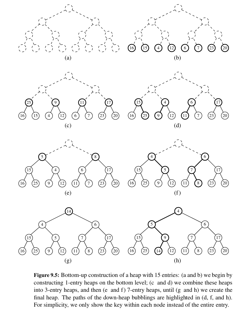
Just know this:

Bottom-up construction of a heap with n entries takes O(n) time, assuming two keys can be compared in O(1) time.

I think heapify works like this ?

Signature: heapify(heap, /)
Docstring: Transform list into a heap, in-place, in O(len(heap)) time.
Type:      builtin_function_or_method

Python’s heapq Module 😍

This part is important.

Python’s standard distribution includes a heapq module that provides support for heap-based priority queues.

That module does not provide any priority queue class; instead it provides functions that allow a standard Python list to be managed as a heap.

Its model is essentially the same as our own, with n elements stored in list cells \(L[0]\) through \(L[n − 1]\), based on the level-numbering indices with the smallest element at the root in \(L[0]\).

We note that heapq does not separately manage associated values; elements serve as their own key.

The heapq module supports the following functions, all of which presume that existing list L satisfies the heap-order property prior to the call:

Method	Explained
heappush(L, e)	Push element e onto list L and restore the heap-order property. The function executes in \(O(log n)\) time.
heappop(L)	Pop and return the element with smallest value from list L, and reestablish the heap-order property. The operation executes in \(O(log n)\) time.
heappushpop(L, e)	Push element e on list L and then pop and return the smallest item. The time is \(O(log n)\), but it is slightly more efficient than separate calls to push and pop because the size of the list never changes. If the newly pushed element becomes the smallest, it is immediately returned. Otherwise, the new element takes the place of the popped element at the root and a down-heap is performed.
heapreplace(L, e)	Similar to heappushpop, but equivalent to the pop being performed before the push (in other words, the new element cannot be returned as the smallest). Again, the time is \(O(log n)\), but it is more efficient that two separate operations. The module supports additional functions that operate on sequences that do not previously satisfy the heap-order property.
heapify(L)	Transform unordered list to satisfy the heap-order property. This executes in \(O(n)\) time by using the bottom-up construction algorithm.
nlargest(k, iterable)	Produce a list of the k largest values from a given iterable. This can be implemented to run in \(O(n + k log n)\) time, where we use n to denote the length of the iterable.
nsmallest(k, iterable)	Produce a list of the k smallest values from a given iterable. This can be implemented to run in \(O(n + k log n)\) time, using similar technique as nlargest.

Sorting with a Priority Queue

Selection-Sort and Insertion-Sort

You can do sorting using priority queues:

Insert all elements to a PQ remove_min 1 by 1.

def pq_sort(C):
    n = len(C)
    p = PriorityQueue()

    # add
    for j in range(n):
        element = C.delete(C.first())
        p.add(element, element)
    # remove
    for j in range(n):
        (k, v) = p.remove_min()
        C.add_last(v)

Selection Sort - \(O(n^2)\) Time Complexity

TODO: Not urgent

...

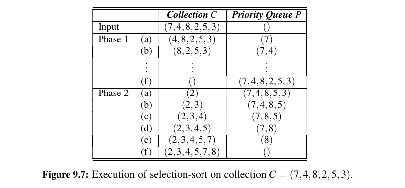
If we implement P with an unsorted list, then Phase 1 of pq_sort takes \(O(n)\) time, for we can add each element in \(O(1)\) time. In Phase 2, the running time of each remove_min operation is proportional to the size of P.

Thus, the bottleneck computation is the repeated “selection” of the minimum element in Phase 2. For this reason, this algorithm is better known as ==selection-sort==.

As noted above, the bottleneck is in Phase 2 where we repeatedly remove an entry with smallest key from the priority queue P. The size of P starts at n and incrementally decreases with each remove_min until it becomes 0.

Thus, the first operation takes time \(O(n)\), the second one takes time \(O(n − 1)\), and so on. Therefore, the total time needed for the second phase is \(O(n^2)\).

Selection Sort on a Collection

Here is an implementation for SelectionSort:

def selection_sort(collection):
    # unsorted list as priority queue
    pq = []
    for _ in range(len(collection)):
        pq.append(collection.pop())

    # find the smallest value and append it back to collection
    for _ in range(len(pq)):
        temp = min(pq)
        collection.append(temp)
        pq.remove(temp)

    return collection

selection_sort([1,5,2,4,9,3,2]) # [1, 2, 2, 3, 4, 5, 9]

Insertion Sort - \(O(n^2)\) Time Complexity

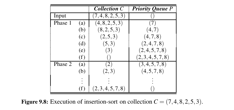
If we implement the priority queue P using a sorted list, then we improve the running time of Phase 2 to \(O(n)\), for each remove_min operation on P now takes \(O(1)\) time.

Unfortunately, Phase 1 becomes the bottleneck for the running time, since, in the worst case, each add operation takes time proportional to the current size of P.

This sorting algorithm is better known as ==insertion-sort== (see Figure 9.8); in fact, our implementation for adding an element to a priority queue is almost identical to a step of insertion-sort as presented in Section 7.5.

The worst-case running time of Phase 1 of insertion-sort is worst-case \(O(n^2)\) time for Phase 1, and thus, the entire insertion-sort algorithm.

However, unlike selection-sort, insertion-sort has a best-case running time of \(O(n)\) (which is kinda irrelevant, but yeah).

Insertion Sort on a Collection

Here is an implementation of Insertion Sort:

def insertion_sort(collection):
    # a sorted list as a priority queue
    pq = []
    for _ in range(len(collection)):
        pq.append(collection.pop())

    # because we will just pop it from this list,
    # let it be sorted in reverse order
    pq.sort(reverse=True)

    for _ in range(len(pq)):
        collection.append(pq.pop())

    return collection

insertion_sort([10,23,6,5,18,23,4]) # [4, 5, 6, 10, 18, 23, 23]

Heap-Sort - \(O(n*log(n))\) Time Complexity - inplacesorting

You can also do sorting using a heap. This is a better sorting than a simple bubble_sort.

Reminder, this was the bubble_sort:

def bubble_sort(collection):
    # start from 0
    for i in range(len(collection)):
        # start from 1
        for j in range(i + 1 , len(collection)):
            if collection[i] > collection[j]:
                collection[i], collection[j] = collection[j], collection[i]
    return collection

bubble_sort([1,34,3,2,56,8,9,55,10]) # [1, 2, 3, 8, 9, 10, 34, 55, 56]

TODO:

...

Here is the most basic implementation of heap sort:

from heapq import heappop, heapify
def heap_sort(collection):
    result = []
    heapify(collection)
    while collection:
        result.append(heappop(collection))
    return result

heap_sort([1,2,7,8,5,2,3,4,6,2]) # [1, 2, 2, 2, 3, 4, 5, 6, 7, 8]

This is an example from REAL WORLD:

from heapq import heapify, heappop, heapreplace
from time import perf_counter_ns
class Solution:
    def heap_sort(self, col: list):
        # o(n)
        heapify(col)
        result = []
        # o(n(logn))
        for i in range(len(col)):
            result.append(heappop(col))
        return result

sol = Solution()
a = perf_counter_ns()

for _ in range(int(1e6)):
    sol.heap_sort([51234,43,1234,51,234,51,2,3,57,9,4,1])

b = perf_counter_ns()

print(f"Method average complication time {(b - a) / int(1e6)}")

Adaptable Priority Queues

Remove randomly from Queue or add VIP.

We need new methods - update() - change priority. - remove() - remove from arbitrary.

Same efficiency -> \(o(log(n))\) for update - remove.

Operation	Running Time
len(p), p.is_empty(), p.min()	\(O(1)\)
p.add(k, v)	\(O(logn)^*\)
p.update(loc, k, v)	\(O(logn)\)
p.remove(loc, )	\(O(logn)^*\)
p.remove_min()	\(O(logn)^*\)

One smart idea:

def _bubble(self, j):
    if j > 0 and self._data[j] < self._data[self._parent(j)]:
        self._upheap(j)
    else:
        self._downheap(j)

...

Locators

TODO: Not urgent

...

Implementing an Adaptable Priority Queue

TODO: Not urgent

...

Fantastic work! 💛 Let's check out Maps, Hash Tables and Skip Lists now.