Memory Management and B-Trees 💕

Our study of data structures thus far has focused primarily upon the efficiency of computations, as measured by the number of primitive operations that are executed on a central processing unit (CPU).

In practice, the performance of a computer system is also greatly impacted by the management of the computer’s memory systems.

In our analysis of data structures, we have provided asymptotic bounds for the overall amount of memory used by a data structure.

In this chapter, we consider more subtle issues involving the use of a computer’s memory system.

The 2 core components

We first discuss ways in which memory is allocated and deallocated during the execution of a computer program, and the impact that this has on the program’s performance.

Second, we discuss the complexity of multilevel memory hierarchies in today’s computer systems.

Although we often abstract a computer’s memory as consisting of a single pool of interchangeable locations, in practice, the data used by an executing program is stored and transferred between a combination of physical memories (e.g., CPU registers, caches, internal memory, and external memory).

We consider the use of classic data structures in the algorithms used to manage memory, and how the use of memory hierarchies impacts the choice of data structures and algorithms for classic problems such as searching and sorting.

Memory Management

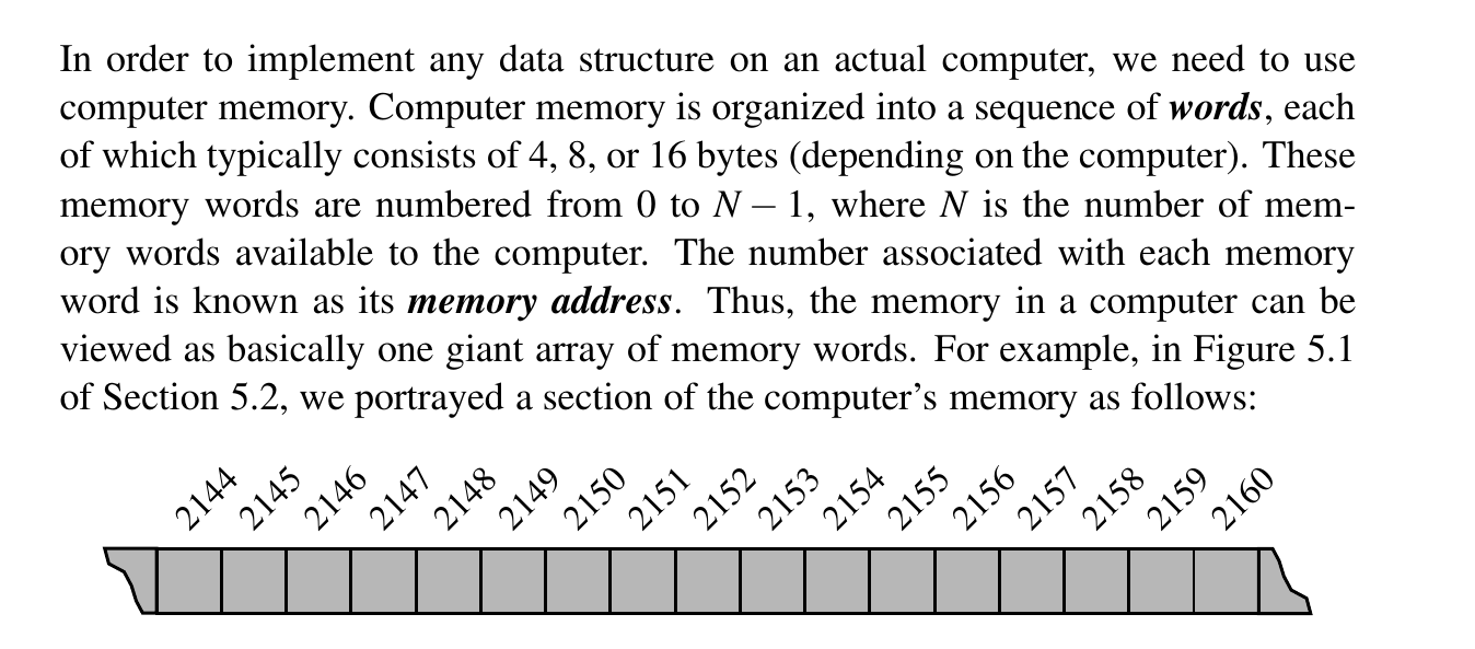
Computer memory is organized into a sequence of words.

The number associated with each memory is the memory address. It is one giant array!

Computer Memory

In order to run programs and store information, computers memory must be managed so as to determine which data is stored in what memory cells.

Memory Allocation

With Python, all objects are stored in a pool of memory, known as the memory heap or Python heap (which should not be confused with the “heap” data structure presented in Chapter 9).

They have the same name but they really aren't similar (even conceptually). A memory heap is called a heap in the same way you would refer to a laundry basket as a "heap of clothes". This name is used to indicate a somewhat messy place where memory can be allocated and deallocated at will. The data structure (as the Wikipedia link you reference points out) is quite different.

When a command such as

w = Widget()

This is executed, assuming Widget is the name of a class, a new instance of the class is created and stored somewhere within the memory heap.

The Python interpreter is responsible for negotiating the use of space with the operating system and for managing the use of the memory heap when executing a Python program.

Fragmentation

Memory allocation in a heap, where memory is divided into contiguous blocks and managed through a linked list called the free list.

As memory is allocated and deallocated, the collection of holes in the free lists changes, with the unused memory being separated into disjoint holes divided by blocks of used memory.

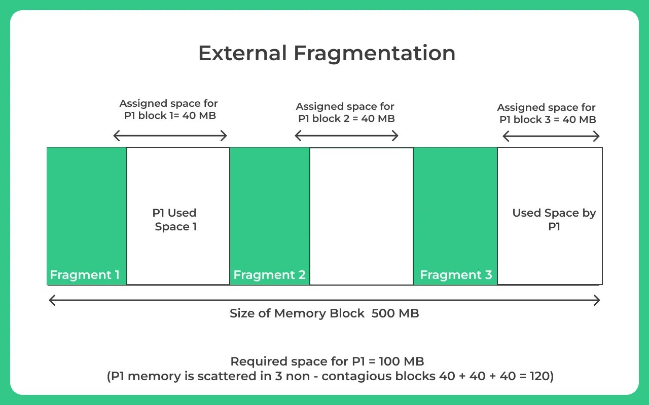
This separation of unused memory into separate holes is known as fragmentation.

Internal Fragmentation

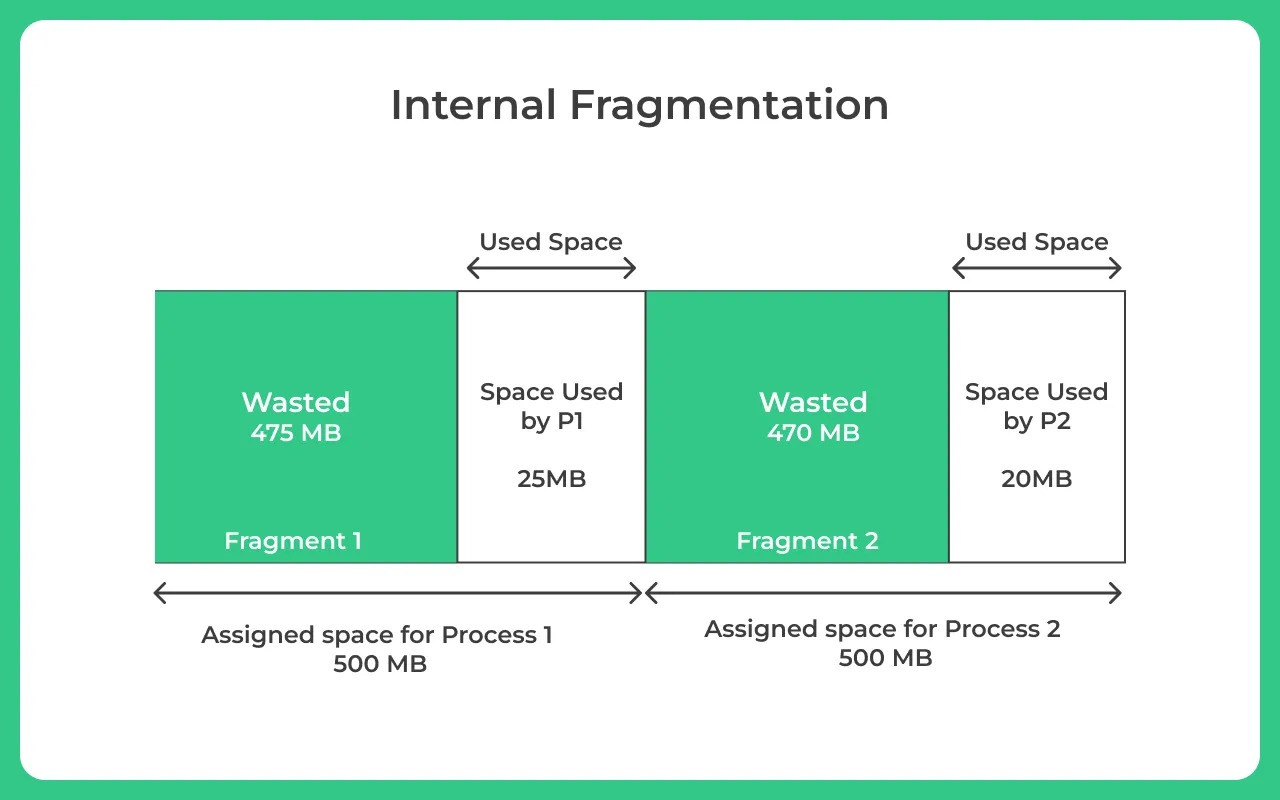
The goal is to minimize fragmentation, which can be internal (unused space within allocated blocks) or external (gaps between allocated blocks).

External Fragmentation

Various allocation algorithms, such as best-fit, first-fit, next-fit, and worst-fit, are introduced.

Best-fit tends to produce more external fragmentation, first-fit causes fragmentation at the front of the free list, next-fit spreads fragmentation but makes large allocations difficult, and worst-fit aims to maintain large contiguous sections of free memory to address fragmentation issues.

The choice of algorithm depends on the trade-offs between speed and fragmentation.

Garbage Collection

George said, this changed everything.

In some languages, like C and C++, the memory space for objects must be explicitly deallocated by the programmer, which is a duty often overlooked by beginner programmers and is the source of frustrating programming errors even for experienced programmers.

The designers of Python instead placed the burden of memory management entirely on the interpreter.

The process of detecting “stale” objects, deallocating the space devoted to those objects, and returning the reclaimed space to the free list is known as garbage collection.

Let the GC handle it

To perform automated garbage collection, there must first be a way to detect those objects that are no longer necessary.

Since the interpreter cannot feasibly analyze the semantics of an arbitrary Python program, it relies on the following conservative rule for reclaiming objects.

In order for a program to access an object, it must have a direct or indirect reference to that object.

We will define such objects to be live objects.

In defining a live object, a direct reference to an object is in the form of an identifier in an active namespace (i.e., the global namespace, or the local namespace for any active function).

For example, immediately after the command w = Widget() is executed, identifier w will be defined in the current namespace as a reference to the new widget object.

We refer to all such objects with direct references as root objects.

An indirect reference to a live object is a reference that occurs within the state of some other live object.

For example, if the widget instance in our earlier example maintains a list as an attribute, that list is also a live object (as it can be reached indirectly through use of identifier w).

The set of live objects are defined recursively; thus, any objects that are referenced within the list that is referenced by the widget are also classified as live objects.

The Python interpreter assumes that live objects are the active objects currently being used by the running program; these objects should not be deallocated. Other objects can be garbage collected.

Reference Counts

Within the state of every Python object is an integer known as its reference count.

This is the count of how many references to the object exist anywhere in the system.

Every time a reference is assigned to this object, its reference count is incremented, and every time one of those references is reassigned to something else, the reference count for the former object is decremented.

The maintenance of a reference count for each object adds \(O(1)\) space per object, and the increments and decrements to the count add \(O(1)\) additional computation time per such operations.

The Python interpreter allows a running program to examine an object’s reference count.

Within the sys module there is a function named getrefcount that returns an integer equal to the reference count for the object sent as a parameter.

It is worth noting that because the formal parameter of that function is assigned to the actual parameter sent by the caller, there is temporarily one additional reference to that object in the local namespace of the function at the time the count is reported.

The advantage of having a reference count for each object is that if an object’s count is ever decremented to zero, that object cannot possibly be a live object and therefore the system can immediately deallocate the object (or place it in a queue of objects that are ready to be deallocated).

Cycle Detection

Cycle detection handles cases where objects still reference each other but can’t be reached from the root — making them unreachable and eligible for garbage collection.

Having a nonzero reference count doesn't guarantee an object's liveness.

Objects can form interconnected groups with references among themselves, making them collectively unreachable from a root object.

An example is given where a list, even with a nonzero reference count, may become garbage collected if the identifier referencing it goes out of scope.

To address such cases, advanced garbage collection methods, like the mark-sweep algorithm, are employed periodically, especially when memory becomes scarce.

These algorithms detect and collect unreachable objects, even when their reference counts are nonzero, preventing memory leaks.

The specifics of garbage collection in Python are abstracted in the gc module and may vary depending on the interpreter's implementation.

Mark and Sweep Algorithm

In the mark-sweep garbage collection algorithm, each object is associated with a "mark" bit to determine liveness. When garbage collection is initiated, all mark bits are cleared.

The algorithm then marks root objects as "live" and performs a depth-first search on the object references, identifying and marking all live objects. This is the "mark" phase.

Subsequently, the algorithm scans the memory heap, reclaiming space used by unmarked objects, and may coalesce allocated space to eliminate external fragmentation temporarily. This scanning and reclamation constitute the "sweep" phase.

The algorithm, which reclaims space proportionate to the number of live objects, their references, and the memory heap size, is efficient in managing memory usage.

DFS In Place 😮

TODO: not urgent.

...

Additional Memory Used by Python Interpreter

We have discussed, in Chapter 15.1.1, how the Python interpreter allocates memory for objects within a memory heap.

However, this is not the only memory that is used when executing a Python program. In this section, we discuss some other important uses of memory.

Run Time Call Stack

Stacks have a most important application to the run-time environment of Python programs.

A running Python program has a private stack, known as the call stack or Python interpreter stack, that is used to keep track of the nested sequence of currently active (that is, non terminated) invocations of functions.

Each entry of the stack is a structure known as an activation record or frame, storing important information about an invocation of a function.

Example CPython behaviour

Here is the talk that this capture is recorded.

import dis

def add(x, y):
    z = x + y 
    return z - 1

dis.dis(add)

  3           0 RESUME                   0

  4           2 LOAD_FAST                0 (x)
              4 LOAD_FAST                1 (y)
              6 BINARY_OP                0 (+)
             10 STORE_FAST               2 (z)

  5          12 LOAD_FAST                2 (z)
             14 LOAD_CONST               1 (1)
             16 BINARY_OP               10 (-)
             20 RETURN_VALUE

At the top of the call stack is the activation record of the running call, that is, the function activation that currently has control of the execution.

The remaining elements of the stack are activation records of the suspended calls, that is, functions that have invoked another function and are currently waiting for that other function to return control when it terminates.

The order of the elements in the stack corresponds to the chain of invocations of the currently active functions.

When a new function is called, an activation record for that call is pushed onto the stack.

When it terminates, its activation record is popped from the stack and the Python interpreter resumes the processing of the previously suspended call.

Each activation record includes a dictionary representing the local namespace for the function call. (See Chapter 1.10 and 2.5 for further discussion of namespaces).

The namespace maps identifiers, which serve as parameters and local variables, to object values, although the objects being referenced still reside in the memory heap.

The activation record for a function call also includes a reference to the function definition itself, and a special variable, known as the program counter, to maintain the address of the statement within the function that is currently executing.

When one function returns control to another, the stored program counter for the suspended function allows the interpreter to properly continue execution of that function.

Recursion

One of the benefits of using a stack to implement the nesting of function calls is that it allows programs to use recursion.

Example

A simple example would be calculating factorials.

\(n! = n*(n-1)*(n-2)*(n-3)*...*1\)

First time only n in the activation record. Recursion makes a new activation record.

The function recursively calls itself to compute (n − 1)!, causing a new activation record, with its own namespace and parameter, to be pushed onto the call stack.

In turn, this recursive invocation calls itself to compute (n − 2)!, and so on.

The chain of recursive invocations, and thus the call stack, grows up to size n + 1, with the most deeply nested call being factorial(0), which returns 1 without any further recursion.

Operand Stack

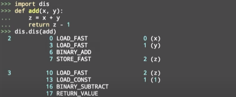
Interestingly, there is actually another place where the Python interpreter uses a stack. Arithmetic expressions, such as ((a + b) ∗ (c + d))/e, are evaluated by the interpreter using an operand stack.

A simple binary operation, such as a + b, is computed by pushing a on the stack, pushing b on the stack, and then calling an instruction that pops the top two items from the stack, performs the binary operation on them, and pushes the result back onto the stack.

push a, push b push __add__ which pops last 2 elements and adds them.

Memory Hierarchies and Caching

With the increased use of computing in society, software applications must manage extremely large data sets.

Such applications include the processing of online financial transactions, the organization and maintenance of databases, and analyses of customers’ purchasing histories and preferences.

The amount of data can be so large that the overall performance of algorithms and data structures sometimes depends more on the time to access the data than on the speed of the CPU.

Memory Systems

Memory is in a hierarchy.

Memory Hierarchy

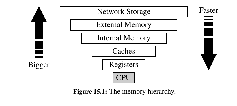
Closest to the CPU are the internal registers that the CPU itself uses.

Access to such locations is very fast, but there are relatively few such locations.

At the second level in the hierarchy are one or more memory caches. This memory is considerably larger than the register set of a CPU, but accessing it takes longer.

At the third level in the hierarchy is the internal memory, which is also known as main memory or core memory. The internal memory is considerably larger than the cache memory, but also requires more time to access.

Another level in the hierarchy is the external memory, which usually consists of disks, CD drives, DVD drives, and/or tapes. This memory is very large, but it is also very slow.

Data stored through an external network can be viewed as yet another level in this hierarchy, with even greater storage capacity, but even slower access.

Caching Strategies

The significance of the memory hierarchy on the performance of a program depends greatly upon the size of the problem we are trying to solve and the physical characteristics of the computer system.

Often, the bottleneck occurs between two levels of the memory hierarchy—the one that can hold all data items and the level just below that one. For a problem that can fit entirely in main memory, the two most important levels are the cache memory and the internal memory.

10 to 100 times longer - cache and internal memory difference 😮

100000 to 10000000 times longer - General Purpose external memory drive. 😮

Most algorithms are not designed with the memory hierarchy in mind, in spite of the great variance between access times for the different levels.

Indeed, all of the algorithm analyses described in this book so far have assumed that all memory accesses are equal.

This assumption might seem, at first, to be a great oversight— and one we are only addressing now in the final chapter—but there are good reasons why it is actually a reasonable assumption to make.

Caching and blocking

Another justification for the memory-access equality assumption is that operating system designers have developed general mechanisms that allow most memory accesses to be fast.

• These mechanisms are based on two important locality-of- reference properties that most software possesses:

  • Temporal locality: If a program accesses a certain memory location, then there is increased likelihood that it accesses that same location again in the near future. For example, it is common to use the value of a counter variable in several different expressions, including one to increment the counter’s value. In fact, a common adage among computer architects is that a program spends 90 percent of its time in 10 percent of its code.

  • Spatial locality: If a program accesses a certain memory location, then there is increased likelihood that it soon accesses other locations that are near this one. For example, a program using an array may be likely to access the locations of this array in a sequential or near-sequential manner.

Temporal and spatial localities have, in turn, given rise to two fundamental design choices for multilevel computer memory systems (which are present in the interface between cache memory and internal memory, and also in the interface between internal memory and external memory).

The first design choice is called virtual memory. This concept consists of providing an address space as large as the capacity of the secondary-level memory, and of transferring data located in the secondary level into the primary level, when they are addressed.

Virtual memory does not limit the programmer to the constraint of the internal memory size.

The concept of bringing data into primary memory is called caching, and it is motivated by temporal locality.

By bringing data into primary memory, we are hoping that it will be accessed again soon, and we will be able to respond quickly to all the requests for this data that come in the near future.

The second design choice is motivated by spatial locality.

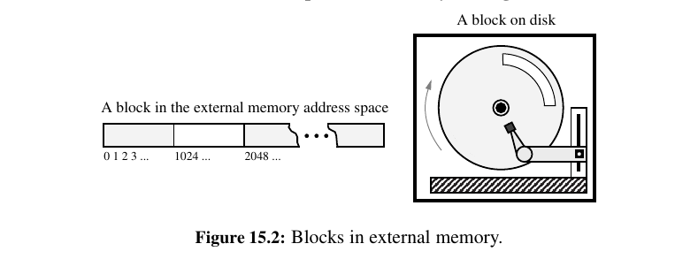
Specifically, if data stored at a secondary-level memory location \(l\) is accessed, then we bring into primary-level memory a large block of contiguous locations that include the location \(l\) (See Figure 15.2.).

This concept is known as blocking, and it is motivated by the expectation that other secondary-level memory locations close to \(l\) will soon be accessed.

In the interface between cache memory and internal memory, such blocks are often called cache lines, and in the interface between internal memory and external memory, such blocks are often called pages.

Blocks in External Memory

Caching in Web Browsers

For motivation, we consider a related problem that arises when revisiting information presented in Web pages.

To exploit temporal locality of reference, it is often advantageous to store copies of Web pages in a cache memory, so these pages can be quickly retrieved when requested again.

This effectively creates a two-level memory hierarchy, with the cache serving as the smaller, quicker internal memory, and the network being the external memory.

In particular, suppose we have a cache memory that has m “slots” that can contain Web pages.

We assume that a Web page can be placed in any slot of the cache. This is known as a fully associative cache.

As a browser executes, it requests different Web pages. Each time the browser requests such a Web page p, the browser determines (using a quick test) if p is unchanged and currently contained in the cache.

If p is contained in the cache, then the browser satisfies the request using the cached copy.

If p is not in the cache, however, the page for p is requested over the Internet and transferred into the cache. If one of the m slots in the cache is available, then the browser assigns p to one of the empty slots.

But if all the m cells of the cache are occupied, then the computer must determine which previously viewed Web page to evict before bringing in p to take its place. There are, of course, many different policies that can be used to determine the page to evict.

Page Replacement Algorithms

• First-in, first-out (FIFO): Evict the page that has been in the cache the longest, that is, the page that was transferred to the cache furthest in the past.

• Least recently used (LRU): Evict the page whose last request occurred furthest in the past.

In addition, we can consider a simple and purely random strategy:

• Random: Choose a page at random to evict from the cache.

Page Replacement Policies

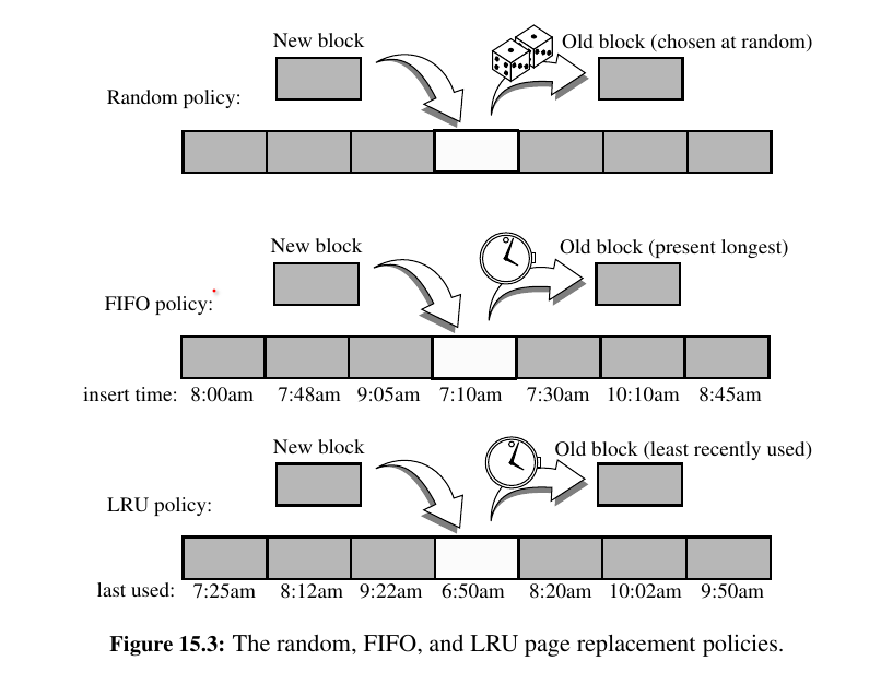
In experiments, best way to approach is: LRU > FIFO > Random

External Searching and B - Trees

Consider the problem of maintaining a large collection of items that does not fit in main memory, such as a typical database.

In this context, we refer to the secondary- memory blocks as disk blocks. Likewise, we refer to the transfer of a block between secondary memory and primary memory as a disk transfer.

Recalling the great time difference that exists between main memory accesses and disk accesses, the main goal of maintaining such a collection in external memory is to minimize the number of disk transfers needed to perform a query or update.

We refer to this count as the I/O complexity of the algorithm involved.

Some Inefficient External-Memory Representations

A typical operation we would like to support is the search for a key in a map.

If we were to store \(n\) items unordered in a doubly linked list, searching for a particular key within the list requires \(n\) transfers in the worst case, since each link hop we perform on the linked list might access a different block of memory.

We can reduce the number of block transfers by using an array-based sequence.

A sequential search of an array can be performed using only \(O(n/B)\) block transfers because of spatial locality of reference, where B denotes the number of elements that fit into a block.

This is because the block transfer when accessing the first element of the array actually retrieves the first B elements, and so on with each successive block.

It is worth noting that the bound of \(O(n/B)\) transfers is only achieved when using a compact array representation (see Chapter 5.2.2).

The standard Python list class is a referential container, and so even though the sequence of references are stored in an array, the actual elements that must be examined during a search are not generally stored sequentially in memory, resulting in n transfers in the worst case.

We could alternately store a sequence using a sorted array. In this case, a search performs \(O(log_{2}n)\) transfers, via binary search, which is a nice improvement.

But we do not get significant benefit from block transfers because each query during a binary search is likely in a different block of the sequence.

As usual, update operations are expensive for a sorted array.

Since these simple implementations are I/O inefficient, we should consider the logarithmic-time internal-memory strategies that use balanced binary trees (which Databases do all the time!) (for example, AVL trees or red-black trees) or other search structures with logarithmic average-case query and update times (for example, skip lists or splay trees).

Typically, each node accessed for a query or update in one of these structures will be in a different block.

Thus, these methods all require \(O(log_{2}n)\) transfers in the worst case to perform a query or update operation.

But we can do better! We can perform map queries and updates using only \(O(log_{B} n) = O(log n/ log B)\) transfers.

(a,b) Trees

To reduce the number of external-memory accesses when searching, we can represent our map using a multiway search tree (Chapter 11.5.1).

This approach gives rise to a generalization of the (2, 4) tree data structure known as the (a, b) tree.

TODO: not urgent

...

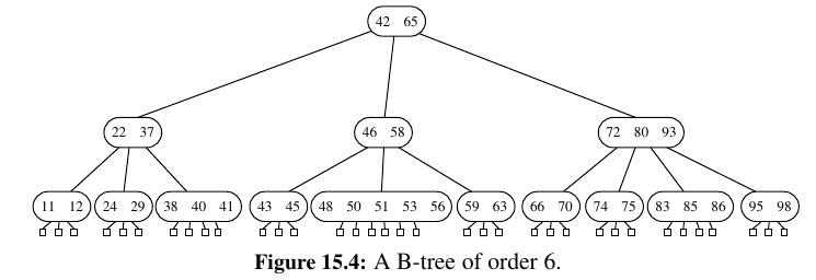
B-Trees

A version of the (a, b) tree data structure, which is the best-known method for maintaining a map in external memory, is called the “B-tree.” (See Figure 15.4.)

A B-tree of order d is an (a, b) tree with \(a = ceil(d/2)\) and \(b = d\).

Since we discussed the standard map query and update methods for (a, b) trees above, we restrict our discussion here to the I/O complexity of B-trees.

B Tree Example

TODO: Not urgent

...

External-Memory Sorting

In addition to data structures, such as maps, that need to be implemented in external memory, there are many algorithms that must also operate on input sets that are too large to fit entirely into internal memory.

In this case, the objective is to solve the algorithmic problem using as few block transfers as possible.

The most classic domain for such external-memory algorithms is the sorting problem.

Multiway Merge-Sort

An efficient way to sort a set S of \(n\) objects in external memory amounts to a simple external-memory variation on the familiar merge-sort algorithm.

The main idea behind this variation is to merge many recursively sorted lists at a time, thereby reducing the number of levels of recursion.

TODO: not urgent

...

Multiway Merging

In a standard merge-sort (Chapter 12.2), the merge process combines two sorted sequences into one by repeatedly taking the smaller of the items at the front of the two respective lists.

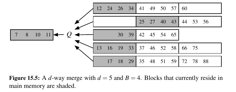
In a d-way merge, we repeatedly find the smallest among the items at the front of the d sequences and place it as the next element of the merged sequence.

We continue until all elements are included. In the context of an external-memory sorting algorithm, if main memory has size M and each block has size B, we can store up to M/B blocks within main memory at any given time.

We specifically choose d = (M/B) − 1 so that we can afford to keep one block from each input sequence in main memory at any given time, and to have one additional block to use as a buffer for the merged sequence. (See Figure 15.5.)

d way merge

TODO: not urgent

...

Unbelievable. You made it to the end. 🎉

I hope you discovered things that will help you in your journey. Onto the next adventure!