Array Based Sequences 🥳¶

This chapter is all about lists, tuples and strings; starting from arrays and dynamic arrays. Which will be the main data structures we'll use. 🎉

Python's Sequence Types¶

In this chapter, we will explore about list, tuple and str classes. Each of them support indexing and accessing to an element within them.

Low - Level Arrays 🥰¶

We have to start with a discussion of the low level computer architecture.

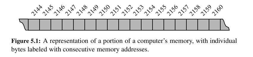
A computer system will have a huge number of bytes of memory, and to keep track of what information is stored in what byte, the computer uses an abstraction known as a memory address.

In effect, each byte of memory is associated with a unique number that serves as it's address (more formally, the binary representation of the number serves as the address).

In this way, the computer system can refer to the data in “byte #2150” versus the data in “byte #2157”

Despite the sequential nature of the numbering system, computer hardware is designed, in theory, so that any byte of the main memory can be efficiently accessed based upon its memory address.

In this sense, we say that a computer’s main memory performs as random access memory (RAM). That is, it is just as easy to retrieve byte #8675309 as it is to retrieve byte #309.

In general, a programming language keeps track of the association between an identifier and the memory address in which the associated value is stored.

A common programming task is to keep track of a sequence of related objects.

For example, we may want a video game to keep track of the top ten scores for that game. Rather than use ten different variables for this task, we would prefer to use a single name for the group and use index numbers to refer to the high scores in that group.

A group of related variables can be stored one after another in a contiguous portion of the computer’s memory. We will denote such a representation as an array.

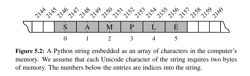
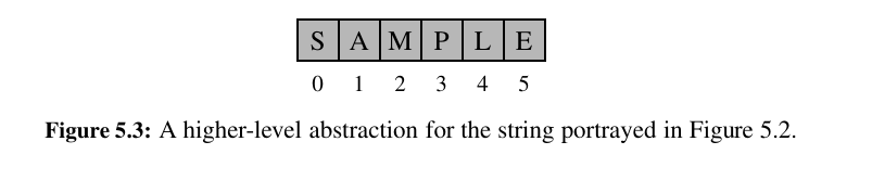
A programmer can envision a high level abstraction to make things easier to work with, like the figure down below for a string:

abstracted_string — A string, abstracted.

Referential Arrays 🤔¶

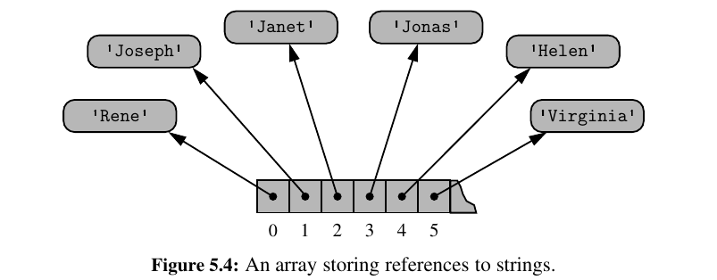
What if we wanted to hold names in an array?

To represent such a list with an array, Python must adhere to the requirement that each cell of the array use the same number of bytes. Yet the elements are strings, and strings naturally have different lengths.

Python could attempt to reserve enough space for each cell to hold the maximum length string (not just of currently stored strings, but of any string we might ever want to store), but that would be wasteful.

Instead, Python represents a list or tuple instance using an internal storage mechanism of an array of object references, which is really cool.

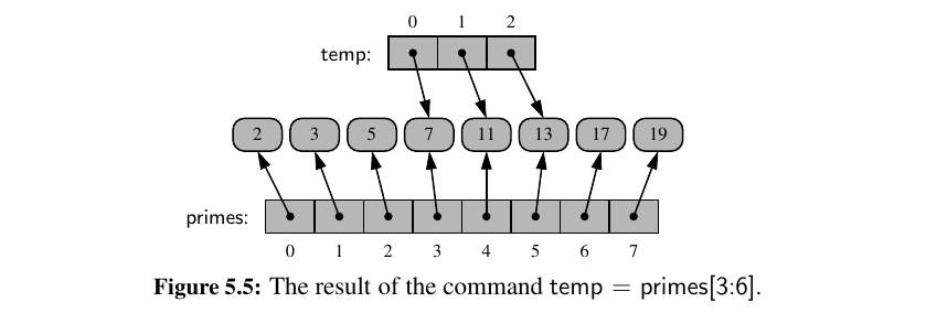
array_of_references — Array of References

When you compute a slice of a list, the result is a new list instance, but that new list has references to the same elements that are in the original list.

The same semantics is demonstrated when making a new list as a copy of an existing one, with a syntax such as backup = list(primes). This produces a new list that is a shallow copy, in that it references the same elements as in the first list.

What happens when we do data = [0] * 8 ?

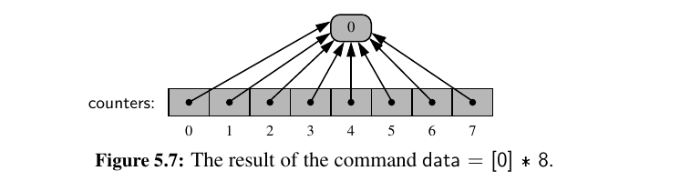
This may seem scary. However, we rely on the fact that the referenced integer is immutable.

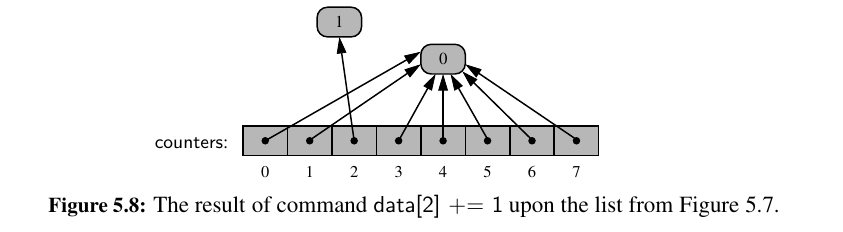
Even a command such as counters[2] += 1 does not technically change the value of the existing integer instance.

This computes a new integer, with value 0 + 1, and sets cell 2 to reference the newly computed value.

Well, how does extend work?

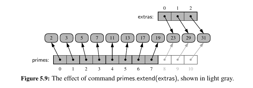
The extended list does not receive copies of those elements, it receives references to those elements.

Compact Arrays in Python¶

In the introduction to this section, we emphasized that strings are represented using an array of characters (not an array of references).

We will refer to this more direct representation as a compact array because the array is storing the bits that represent the primary data (characters, in the case of strings).

The overall memory usage will be much lower for a compact structure because there is no overhead devoted to the explicit storage of the sequence of memory references (in addition to the primary data).

Tip

No need for addresses:

Suppose we wish to store a sequence of one million, 64-bit integers.

In theory, we might hope to use only 64 million bits. However, we estimate that a Python list will use four to five times as much memory.

Each element of the list will result in a 64-bit memory address being stored in the primary array, and an int instance being stored elsewhere in memory.

Tip

Not Near:

Another important advantage to a compact structure for high-performance computing is that the primary data are stored consecutively in memory. Note well that this is not the case for a referential structure.

That is, even though a list maintains careful ordering of the sequence of memory addresses, where those elements reside in memory is not determined by the list.

Because of the workings of the cache and memory hierarchies of computers, it is often advantageous to have data stored in memory near other data that might be used in the same computations.

`array` module¶

Primary support for compact arrays is in a module named array.

import array
primes = array( "i" , [2, 3, 5, 7, 11, 13, 17, 19])

The type code allows the interpreter to determine precisely how many bits are needed per element of the array. The types are based on C programming language.

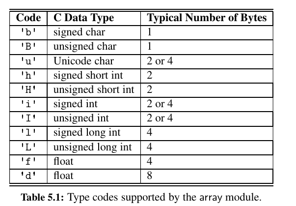
The array module does not provide support for making compact arrays of user-defined data types.

Compact arrays of such structures can be created with the lower-level support of a module named ctypes.

Dynamic Arrays and Amortization 🤔¶

When creating a low-level array in a computer system, the precise size of that array must be explicitly declared in order for the system to properly allocate a consecutive piece of memory for its storage.

Because the system might dedicate neighboring memory locations to store other data, the capacity of an array cannot trivially be increased by expanding into subsequent cells.

In the context of representing a Python tuple or str instance, this constraint is no problem.

Instances of those classes are immutable, so the correct size for an underlying array can be fixed when the object is instantiated.

Python’s list class presents a more interesting abstraction.

Although a list has a particular length when constructed, the class allows us to add elements to the list, with no apparent limit on the overall capacity of the list.

To provide this abstraction, Python relies on an algorithmic sleight of hand known as a dynamic array.

The first key to providing the semantics of a dynamic array is that a list instance maintains an underlying array that often has greater capacity than the current length of the list.

For example, while a user may have created a list with five elements, the system may have reserved an underlying array capable of storing eight object references (rather than only five).

This extra capacity makes it easy to append a new element to the list by using the next available cell of the array. If a user continues to append elements to a list, any reserved capacity will eventually be exhausted.

In that case, the class requests a new, larger array from the system, and initializes the new array so that its prefix matches that of the existing smaller array.

At that point in time, the old array is no longer needed, so it is reclaimed by the system.

Intuitively, this strategy is much like that of the hermit crab, which moves into a larger shell when it outgrows its previous one. Yep you heard that right. Lists are hermit crabs.

import sys   # provides getsizeof function
data = []
for k in range(n):   # NOTE: must fix choice of n
    a = len(data)    # number of elements
    b = sys.getsizeof(data) # actual size in bytes
    print("Length: {0:3d}; Size in bytes: {1:4d}".format(a, b))
    data.append(None) # increase length by one

Length: 0; Size in bytes :  72
Length: 1; Size in bytes : 104
Length: 2; Size in bytes : 104
Length: 3; Size in bytes : 104
Length: 4; Size in bytes : 104
Length: 5; Size in bytes : 136
Length: 6; Size in bytes : 136
Length: 7; Size in bytes : 136
Length: 8; Size in bytes : 136
Length: 9; Size in bytes : 200
Length: 10; Size in bytes : 200
Length: 11; Size in bytes : 200
Length: 12; Size in bytes : 200

We see that an empty list instance already requires a certain number of bytes of memory (72 on our system). This is only the memory allocated by the list itself, not elements.

As soon as the first element is inserted into the list, we detect a change in the underlying size of the structure.

In particular, we see the number of bytes jump from 72 to 104, an increase of exactly 32 bytes. Our experiment was run on a 64-bit machine architecture, meaning that each memory address is a 64-bit number (i.e., 8 bytes).

We speculate that the increase of 32 bytes reflects the allocation of an underlying array capable of storing four object references.

This hypothesis is consistent with the fact that we do not see any underlying change in the memory usage after inserting the second, third, or fourth element into the list.

Implementing a Dynamic Array 🤔¶

How would we do it? See the code down below:

dynamic_array.py
import ctypes                                   # provides low-level arrays

class DynamicArray:
    """A dynamic array class akin to a simplified Python list."""
    def __init__(self):
        """Create an empty array."""
        self._n = 0                                 # count actual elements
        self._capacity = 1                          # default array capacity
        self._A = self._make_array(self._capacity)  # low-level array

    def __len__ (self):
        """Return number of elements stored in the array."""
        return self._n

    def __getitem__ (self, k): 
        """Return element at index k."""
        if not 0 <= k < self._n:
            raise IndexError("invalid index")
        return self._A[k] # retrieve from array

    def append(self, obj): 
        """Add object to end of the array."""
        if self._n == self._capacity: # not enough room
            self._resize(2 * self._capacity) # so double capacity
        self._A[self._n] = obj
        self._n += 1 

    def _resize(self, c): # nonpublic utitity
        """Resize internal array to capacity c."""
        B = self._make_array(c) # new (bigger) array
        for k in range(self._n): # for each existing value
            B[k] = self._A[k]
        self._A = B # use the bigger array
        self._capacity = c

    def _make_array(self, c): # nonpublic utitity
        """Return new array with capacity c."""
        return (c * ctypes.py_object)( ) # see ctypes documentation

Amortized Analysis of Dynamic Arrays 🤨¶

By doubling the capacity during an array replacement, our new array allows us to add n new elements before the array must be replaced again. In this way, there are many simple append operations for each expensive one (see Figure 5.13).

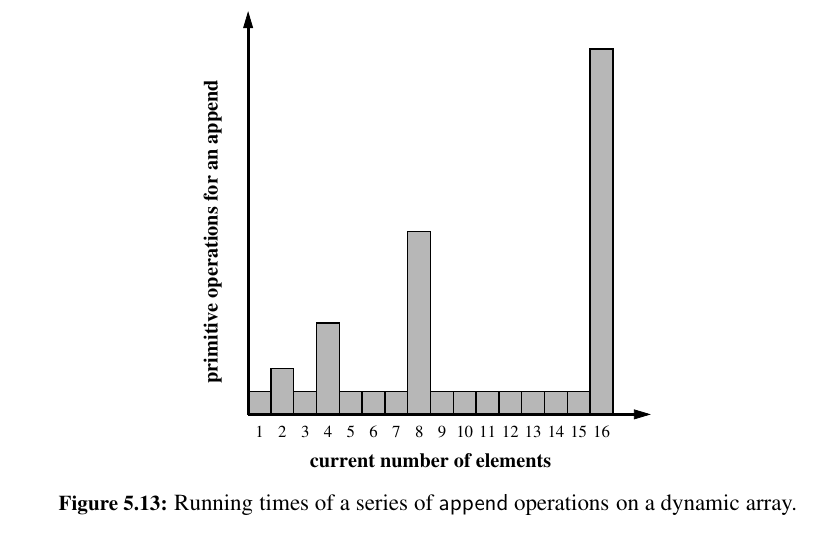
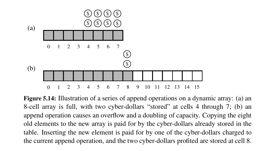
appending_dynamic_array — What happens while appending

Using an algorithmic design pattern called amortization, we can show that performing a sequence of such append operations on a dynamic array is actually quite efficient.

3 dollars for each append, every append that you don't overflow is a profit of 2 dollars. Next big overflow will be using the profit to double the capacity and the math adds up.

Can we approach the problem any other way?

If we instead increase the array by only 25% of its current size (i.e., a geometric base of 1.25), we do not risk wasting as much memory in the end, but there will be more intermediate resize events along the way.

Doubling seems like the optimal approach.

Another consequence of the rule of a geometric increase in capacity when appending to a dynamic array is that the final array size is guaranteed to be proportional to the overall number of elements. That is, the data structure uses \(O(n)\) memory.

This is a very desirable property for a data structure.

If a container, such as a Python list, provides operations that cause the removal of one or more elements, greater care must be taken to ensure that a dynamic array guarantees \(O(n)\) memory usage.

The risk is that repeated insertions may cause the underlying array to grow arbitrarily large, and that there will no longer be a proportional relationship between the actual number of elements and the array capacity after many elements are removed.

A robust implementation of such a data structure will shrink the underlying array, on occasion, while maintaining the \(O(1)\) amortized bound on individual operations.

However, care must be taken to ensure that the structure cannot rapidly oscillate between growing and shrinking the underlying array, in which case the amortized bound would not be achieved.

Python’s List Class 💙¶

["references", "to", "all"]

A careful examination of the intermediate array capacities suggests that Python is not using a pure geometric progression, nor is it using an arithmetic progression.

from time import time
def compute_average(n):
    """Perform n appends to an empty list and return average time elapsed."""
    data = []
    start = time()
    for k in range(n):
        data.append(None)
    end = time()
    return end - start / n

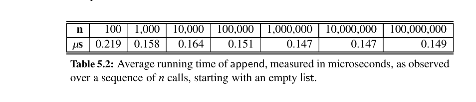
Append is getting faster which is expected with less doubling/expanding in size:

avg_run_time_append — Average Running Time for Append

Efficiency of Python's Sequence Types¶

How about the efficiency of other sequence types of Python? Here are some non mutating methods used by lists and tuples.

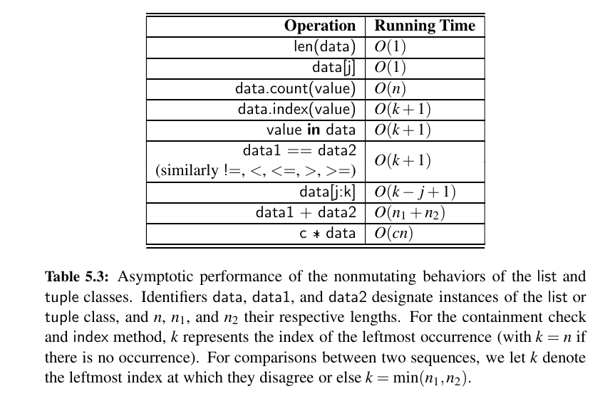
Tuples are typically more memory efficient. 👨‍💻

Here are some mutating behaviors:

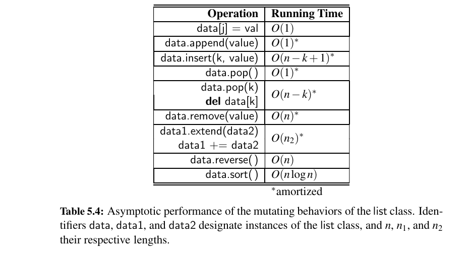
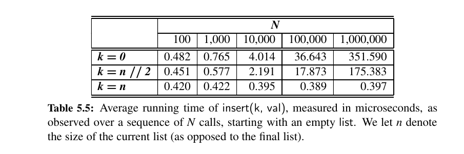
First thing you see is to append a list from the end is better than to be doing that from beginning or the start. You can see the difference here:

"""3 different cases"""
for n in range(N):
    data.insert(0, None)

for n in range(N):
    data.insert(n//2, None)

for n in range(N):
    data.insert(n, None)

avg_run_time_insert — Average Running Time for Insert

Secondly, popping from the end is really fast (\(O(1)\) amortized) but the middle or start is, oh no.

removing_from_middle — Removing From Middle

Also remove(element) is just a disaster. Traverse the whole list, find the element, remove it. No efficient way here.

Extending a list is just appending hidden under a mask 😉

In effect, a call to data.extend(other) produces the same outcome as the code:

for element in other:
    data.append(element)

Running time is proportional to the length of the other list.

So why would you want to call l1.extend(l2) ?

There is always some advantage to using an appropriate Python method, because those methods are often implemented natively in a compiled language (rather than as interpreted Python code).

Secondly, there is less overhead to a single function call that accomplishes all the work, versus many individual function calls.

Finally, for making a list, list comprehension is significantly faster than building a list and appending:

n = 73
squares = [elem * elem for elem in range(1, n+1)]

Tip

There is one thisg you might find yourself doing over and over again, and it's the topic of reversing a list ?

Here are some guidelines on it:

a = ["a", "b", "c", "d" , "e"]

for elem in reversed(a):
    print(elem, end = " ") # e d c b a 

print()

for i in range(len(a) - 1, -1 , -1):
    print(a[i], end = " ") # e d c b a 

print()

for elem in a[::-1]:
    print(elem, end = " ") # e d c b a 

print()

# The list. reverse() method reverses the elements of the 
# list in place. The method returns None because it 
# mutates the original list. 
a.reverse()
for elem in a:
    print(elem, end= " ") # e d c b a 

print()
print("This is not good, a changed")

Python's String Class¶

"fn_Believed!"

We learned about strings in Chapter 1. Here is how they are analyzed:

The analysis for many behaviors is quite intuitive.

For example, methods that produce a new string (e.g., capitalize, center, strip) require time that is linear in the length of the string that is produced.

Many of the behaviors that test Boolean conditions of a string (e.g., islower) take \(O(n)\) time, examining all \(n\) characters in the worst case, but short circuiting as soon as the answer becomes evident (e.g., islower can immediately return False if the first character is upper cased).

The comparison operators (e.g., ==, <) fall into this category as well.

Some of the most interesting behaviors, from an algorithmic point of view, are those that in some way depend upon finding a string pattern within a larger string; this goal is at the heart of methods such as __contains__ , find, index, count, replace, and split.

We will dive deep in Chapter 13.

Composing Strings¶

Doing repeated concatenation is terribly inefficient.

Warning

Do not do this:

letters = ""
for c in document:
    if c.isalpha():
        letters += c

Constructing the new string would require time proportional to its length.

If the final result has n characters, the series of concatenations would take time proportional to the familiar sum \(1 + 2 +3 + · · · + n\) , and therefore \(O(n^{2})\) time.

Instead - Use lists - strings with split and join. 🎋

Because appending to end of a list is \(O(1)\).

temp = []  # start with empty list
for c in document:
    if c.isalpha():
        temp.append(c)  # append alphabetic character
letters = "".join(temp)  # compose overall result

Or even better:

letters = "".join([c for c in document if c.isalpha()])
# not even a list is needed
letters = "".join(c for c in document if c.isalpha())

Using Array Based Sequences 😍¶

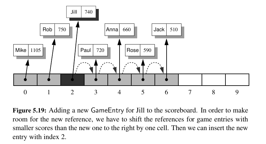
We talked about leader boards.

To maintain a sequence of high scores, we develop a class named Scoreboard.

Here is a complete Python implementation of the Scoreboard and NewScore class.

scoreboard.py
class Scoreboard:
    """Fixed length sequence of high scores in nondecreasing order"""
    def __init__(self, capacity=10):
        """Initialize scoreboard with given maximum capacity
        All initial entries are None"""
        self._board = [None] * capacity
        self._n = 0

    def __getitem__(self, k):
        """Return entry at index k"""
        return self._board[k]

    def __str__(self):
        """Return string representation of the high score list"""
        return "\n".join(str(entry) for entry in self._board if entry is not None)

    def __len__(self):
        return self._n

    def add(self, entry):
        """Consider adding entry to high scores"""
        score = entry.get_score()

        # Does this entry qualify as high score?
        # answer is yes if board not full or score is higher than last entry
        # if we have room or if we have a new high score,
        # leaderboard should be updated.
        good = self._n < len(self._board) or score > self._board[-1].get_score()

        if good:
            if self._n < len(self._board):
                self._n += 1
            # shift lower scores rightward to make room for new entry
            j = self._n - 1
            while j > 0 and self._board[j-1] is not None and self._board[j-1].get_score() < score:
                self._board[j] = self._board[j-1]
                j -= 1
            self._board[j] = entry

class NewScore:
    def __init__(self, name: str, score: int):
        self._name = name
        self._score = score

    def get_score(self):
        return self._score

    def get_name(self):
        return self._name

    def __repr__(self):
        return f"{self._name} scored {self._score}"

world = Scoreboard()

score1 = NewScore("Sumail", 400)
score2 = NewScore("Micke", 700)
score3 = NewScore("Arteezy", 800)
score4 = NewScore("Zai", 570)

world.add(score1)
world.add(score2)
world.add(score3)
world.add(score4)

print(world)

# Arteezy scored 800 
# Micke scored 700 
# Zai scored 570 
# Sumail scored 400

Sorting a Sequence 💎¶

Sorting is crucial. If something is sorted, it is really easier to index it.

Insertion Sort¶

start from 1 - slap city 🎩

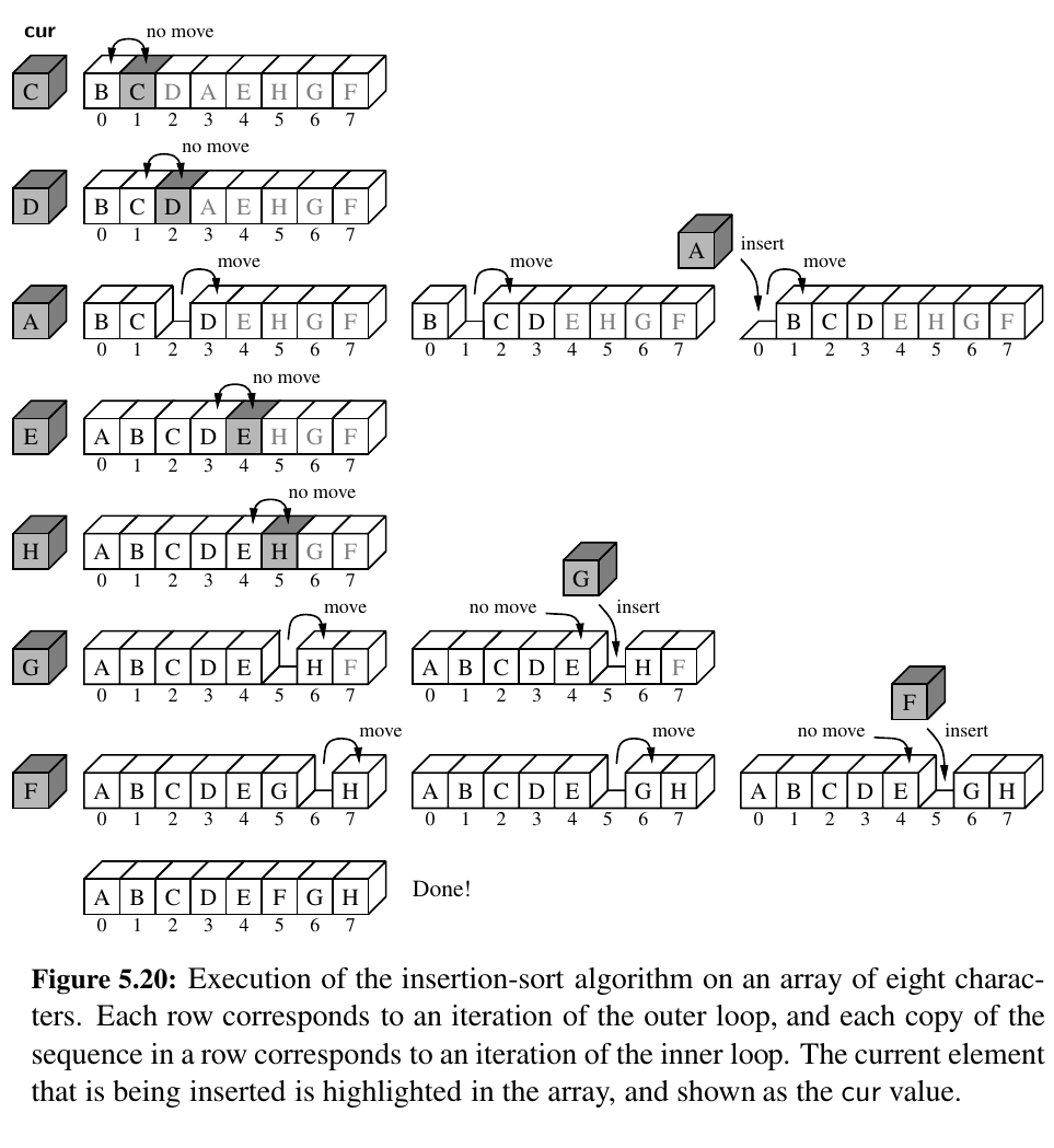
We study several sorting algorithms in this book, most of which are described in Chapter 12. As a warm-up, in this section we describe a nice, simple sorting algorithm known as insertion-sort.

• We start with the first element in the array. One element by itself is already sorted.

• Then we consider the next element in the array. If it is smaller than the first, we swap them.

• Next we consider the third element in the array. We swap it leftward until it is in its proper order with the first two elements.

• We then consider the fourth element, and swap it leftward until it is in the proper order with the first three.

• We continue in this manner with the fifth element, the sixth, and so on, until the whole array is sorted.

Insertion Sort: Compare as you insert. Time complexity is \(O(n^2)\).

insertion_sort.py
def insertionSort(array):
    """Sort elements in a list in non decreasing order"""
    for step in range(1, len(array)):
        key = array[step]
        # index on left
        j = step - 1
        # Compare key with each element on the left of it
        # until an element smaller than it is found
        # For descending order, change key<array[j] to key>array[j].
        while j >= 0 and key < array[j]:
            # slap the value on jth to right neighbour
            array[j + 1] = array[j]
            # decrease j
            j = j - 1
            # run this until you get to the start of the list
            # or you find an element smaller than jth.
            # if the value is bigger just keep slapping.
        # Place key at after the element just smaller than it.
        array[j + 1] = key

data = [9, 5, 1, 4, 3]
insertionSort(data)
print(f'Sorted data: {data}') # Sorted data: [1, 3, 4, 5, 9]

Simple Cryptography 🔎¶

Tip

There is a perfect balance between ord() and chr().

ord() takes a one length string and returns an integer code point for that. chr() takes an int and returns a one length string for it:

print(ord("A")) # 65
print(chr(101)) # e

An interesting application of strings and lists is cryptography, the science of secret messages and their applications.

Encryption: Plain Text to ciphertext.

Decryption: Ciphertext to plain text.

Arguably the earliest encryption scheme is the Caesar cipher, which is named after Julius Caesar, who used this scheme to protect important military messages (All of Caesar’s messages were written in Latin, of course, which already makes them unreadable for most of us!).

The Caesar cipher is a simple way to obscure a message written in a language that forms words with an alphabet.

The Caesar cipher involves replacing each letter in a message with the letter that is a certain number of letters after it in the alphabet.

So, in an English message, we might replace each A with D, each B with E, each C with F, and so on, if shifting by three characters.

We continue this approach all the way up to W, which is replaced with Z. Then, we let the substitution pattern wrap around, so that we replace X with A, Y with B, and Z with C.

Our goal is to achieve this conversation:

Secret: WKH HDJOH LV LQ SODB; PHHW DW MRH’V.
Message: THE EAGLE IS IN PLAY; MEET AT JOE’S.

Here is the CeaserCipher Class:

caesarcipher.py
class CaesarCipher():
    """Class for doing encryption and decryption using CaesarCipher"""
    def __init__(self, shift):
        """Construct CeaselCipher using given integer shift for rotation"""
        encoder = [None] * 26
        decoder = [None] * 26
        for k in range(26):
            # encoder is the secret. a list of chars
            encoder[k] = chr((k+shift) % 26 + ord("A"))
            decoder[k] = chr((k-shift) % 26 + ord("A"))
        self._forward = "".join(encoder)
        self._backward = "".join(decoder)

    def _encrypt(self, message):
        """Return string encrypted by CaesarCipher"""
        return self._transform(message, self._forward)

    def _decrypt(self, secret):
        """Return string decrypted by CaesarCipher"""
        return self._transform(secret, self._backward)

    def _transform(self, original, code):
        """Utility to perform transformation based on given code string."""
        # message in a list
        msg = list(original)
        for k in range(len(msg)):
            if msg[k].isupper():
                j = ord(msg[k]) - ord("A")
                msg[k] = code[j]
        return "".join(msg)

if __name__ == "__main__":
    cipher = CaesarCipher(shift=3)
    message = "THE EAGLE IS IN PLAY, MEET AT JOES"
    coded = cipher._encrypt(message)
    print(f"Secret is : {coded}")
    answer = cipher._decrypt(coded)
    print(f"Message is : {answer}")

Feel free to try this out!

Multidimensional Data Sets 🤭¶

Lists, tuples, and strings in Python are one-dimensional.

We use a single index to access each element of the sequence. Many computer applications involve multidimensional data sets.

For example, computer graphics are often modeled in either two or three dimensions.

Geographic information may be naturally represented in two dimensions, medical imaging may provide three-dimensional scans of a patient, and a company’s valuation is often based upon a high number of independent financial measures that can be modeled as multidimensional data.

A two-dimensional array is sometimes also called a matrix.

For example, the two-dimensional data:

22  18  709  5  33
45  32  830  120 750
4  880  45  66 61

might be stored in Python as follows:

data = [ [22, 18, 709, 5, 33], [45, 32, 830, 120, 750], [4, 880, 45, 66, 61] ]

Constructing a Multidimensional List¶

These are some common mistakes:

data = ([0] * c) * r # this just multiplies the list like concatenation

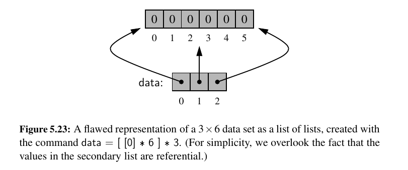
data = [[0] * c] * r 
# this is still wrong because all r entries of list are 
# references to the same instance list of c zeros.
# the visual is down below

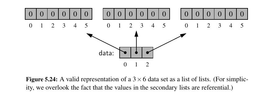
The correct way: LIST COMPREHENSIONS FOR THE RESCUE.

data = [ [0] * c for i in range(r)]

By using list comprehension, the expression [0] * c is reevaluated for each pass of the embedded for loop.

Therefore, we get r distinct secondary lists, as desired (We note that the variable i in that command is irrelevant; we simply need a for loop that iterates r times).

Tic Tac Toe 🥰¶

This game is not even interesting because a good player can always force a tie.

But for just training, here is the code for TicTacToe:

tictactoe.py
class TicTacToe:
    """Management of a Tic-Tac-Toe game (does not do strategy)."""

    def __init__(self):
        """Start a new game."""
        self._board = [[' '] * 3 for j in range(3)]
        self._player = 'X'

    def mark(self, i, j):
        """Put an X or O mark at position (i,j) for next player's turn."""
        if not (0 <= i <= 2 and 0 <= j <= 2):
            raise ValueError('Invalid board position')
        if self._board[i][j] != ' ':
            raise ValueError('Board position occupied')
        if self.winner() is not None:
            raise ValueError('Game is already complete')
        self._board[i][j] = self._player
        if self._player == 'X':
            self._player = 'O'
        else:
            self._player = 'X'

    def _is_win(self, mark):
        """Check whether the board configuration is a win for the given player."""
        board = self._board  # local variable for shorthand
        return (mark == board[0][0] == board[0][1] == board[0][2] or  # row 0
                mark == board[1][0] == board[1][1] == board[1][2] or  # row 1
                mark == board[2][0] == board[2][1] == board[2][2] or  # row 2
                mark == board[0][0] == board[1][0] == board[2][0] or  # column 0
                mark == board[0][1] == board[1][1] == board[2][1] or  # column 1
                mark == board[0][2] == board[1][2] == board[2][2] or  # column 2
                mark == board[0][0] == board[1][1] == board[2][2] or  # diagonal
                mark == board[0][2] == board[1][1] == board[2][0])  # rev diag

    def winner(self):
        """Return mark of winning player, or None to indicate a tie."""
        for mark in 'XO':
            if self._is_win(mark):
                return mark
        return None

    def __str__(self):
        """Return string representation of current game board."""
        rows = ['|'.join(self._board[r]) for r in range(3)]
        return '\n-----\n'.join(rows)


if __name__ == '__main__':
    game = TicTacToe()
    # X moves:            # O moves:
    game.mark(1, 1)
    game.mark(0, 2)
    game.mark(2, 2)
    game.mark(0, 0)
    game.mark(0, 1)
    game.mark(2, 1)
    game.mark(1, 2)
    game.mark(1, 0)
    game.mark(2, 0)

    print(game)
    winner = game.winner()
    if winner is None:
        print('Tie')
    else:
        print(winner, 'wins')

Now, let's move to Stacks, Queues and Dequeues. 💚