All About Trees 🌳
Productivity experts say that breakthroughs come by thinking “non linearly”.
In this chapter, we discuss one of the most important nonlinear data structures in computing—trees.
Tree structures are indeed a breakthrough in data organization, for they allow us to implement a host of algorithms much faster than when using linear data structures, such as array-based lists or linked lists.
Trees also provide a natural organization for data, and consequently have become ubiquitous structures in file systems, graphical user interfaces, databases, Web sites, and other computer systems.
General Trees
The relationships in a tree are hierarchical, with some objects being “above” and some “below” others.
Tree Definitions and Properties
A tree is an abstract data type that stores elements hierarchically.
With the exception of the top element, each element in a tree has a parent element and zero or more children elements.
We typically call the top element the root of the tree, but it is drawn as the highest element, with the other elements being connected below (just the opposite of a botanical tree).
Other Node Relationships - Internal External
Two nodes that are children of the same parent are siblings.
A node v is external if v has no children. A node v is internal if it has one or more children.
External nodes are also known as leaves.
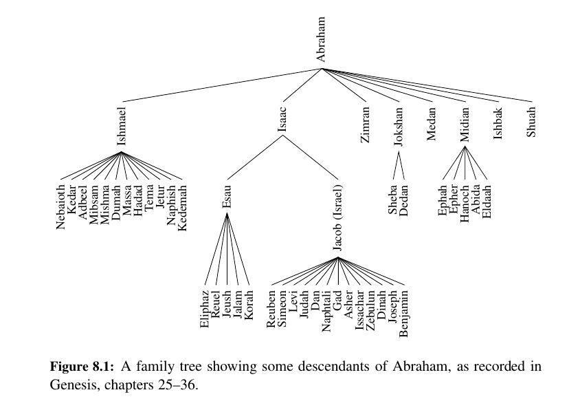
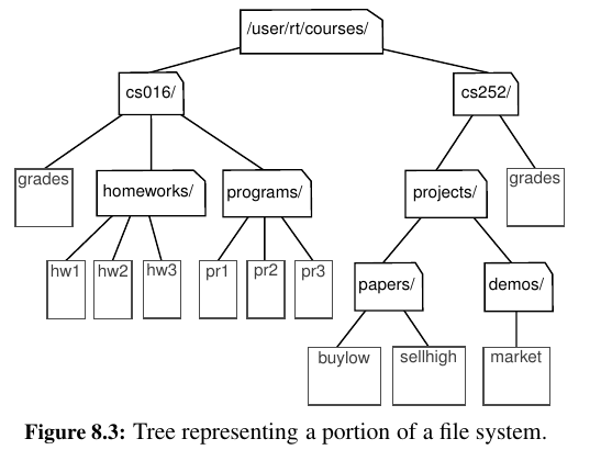
We discussed the hierarchical relationship between files and directories in a computer’s file system, although at the time we did not emphasize the nomenclature of a file system as a tree.
Now we revisit an earlier example. We see that the internal nodes of the tree are associated with directories and the leaves are associated with regular files.
In the UNIX and Linux operating systems, the root of the tree is appropriately called the “root directory,” and is represented by the symbol “/.”
ancestor - descendant
A node u is an ancestor of a node v if u = v or u is an ancestor of the parent of v. Conversely, we say that a node v is a descendant of a node u if u is an ancestor of v.
For example, in Figure 8.3, cs252/ is an ancestor of papers/, and pr3 is a descendant of cs016/.
The sub tree of T rooted at a node v is the tree consisting of all the descendants of v in T (including v itself).
In Figure 8.3, the sub tree rooted at cs016/ consists of the nodes cs016/, grades, homeworks/, programs/, hw1, hw2, hw3, pr1, pr2, and pr3.
Edges and Paths in Trees
An edge of tree T is a pair of nodes (u, v) such that u is the parent of v, or vice versa.
A path of T is a sequence of nodes such that any two consecutive nodes in the sequence form an edge.
For example, the tree in Figure 8.3 contains the path (cs252/, projects/, demos/, market).
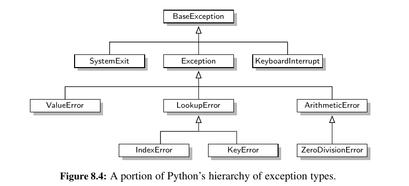
The inheritance relation between classes in a Python program forms a tree when single inheritance is used. For example, in Chapter 2.4 we provided a summary of the hierarchy for Python’s exception types, as portrayed in Figure 8.4.
The BaseException class is the root of that hierarchy, while all user-defined exception classes should conventionally be declared as descendants of the more specific Exception class.
Wisdom:
In Python, all classes are organized into a single hierarchy, as there exists a built-in class named object as the ultimate base class.
It is a direct or indirect base class of all other types in Python (even if not declared as such when defining a new class). Therefore, the hierarchy pictured in Figure 8.4 is only a portion of Python’s complete class hierarchy.
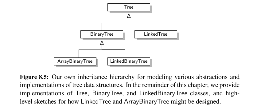
As a preview of the remainder of this chapter, Figure 8.5 portrays our own hierarchy of classes for representing various forms of a tree.
Ordered Trees
A tree is ordered if there is a meaningful linear order among the children of each node; that is, we purposefully identify the children of a node as being the first, second, third, and so on.
Such an order is usually visualized by arranging siblings left to right, according to their order.
A book, are hierarchically organized as a tree whose internal nodes are parts, chapters, and sections, and whose leaves are paragraphs, tables, figures, and so on.
The Tree Abstract Data Type
An element is stored at each position, and positions satisfy parent-child relationships that define the tree structure. A position object for a tree supports the method:
p.element(): Return the element stored at position p.
The tree ADT then supports the following accessor methods, allowing a user to navigate the various positions of a tree:
| Method | Explained |
|---|---|
T.root() |
Return the position of the root of tree T, or None if T is empty. |
T.is_root(p) |
Return True if position p is the root of Tree T. |
T.parent(p) |
Return the position of the parent of position p, or None if p is the root of T. |
T.num_children(p) |
Return the number of children of position p. |
T.children(p) |
Generate an iteration of the children of position p. |
T.is_leaf(p) |
Return True if position p does not have any children. |
len(T) |
Return the number of positions (and hence elements) that are contained in tree T. |
T.is_empty() |
Return True if tree T does not contain any positions. |
T.positions() |
Generate an iteration of all positions of tree T. |
iter(T) |
Generate an iteration of all elements stored within tree T. |
If a tree T is ordered, then T.children(p) reports the children of p in the natural order.
If p is a leaf, then T.children(p) generates an empty iteration.
In similar regard, if tree T is empty, then both T.positions() and iter(T) generate empty iterations.
A Tree Abstract Base Class in Python
In discussing the object-oriented design principle of abstraction in Chapter 2, we noted that a public interface for an abstract data type is often managed in Python via duck typing.
For example, we defined the notion of the public interface for a queue ADT in Chapter 6, and have since presented several classes that implement the queue interface (e.g., ArrayQueue in Chapter 6, LinkedQueue and CircularQueue in Chapter 7).
However, we never gave any formal definition of the queue ADT in Python; all of the concrete implementations were self-contained classes that just happen to adhere to the same public interface.
A more formal mechanism to designate the relationships between different implementations of the same abstraction is through the definition of one class that serves as an abstract base class, via inheritance, for one or more concrete classes.
We choose to define a Tree class, that serves as an abstract base class corresponding to the tree ADT.
Our reason for doing so is that there is quite a bit of useful code that we can provide, even at this level of abstraction, allowing greater code reuse in the concrete tree implementations we later define.
Although the Tree class is an abstract base class, it includes several concrete methods with implementations that rely on calls to the abstract methods of the class.
We note that, with the Tree class being abstract, there is no reason to create a direct instance of it, nor would such an instance be useful. The class exists to serve as a base for inheritance, and users will create instances of concrete subclasses.
Here is the code:
Computing Depth and Height
Let p be the position of a node of a tree T. The depth of p is the number of ancestors of p, excluding p itself.
Note that this definition implies that the depth of the root of T is 0.
Here is an approach for our Trees:
def depth(self, p):
"""Return the number of levels separating Position p from the root."""
if self.is_root(p):
return 0
else:
return 1 + self.depth(self.parent(p))
The height of a position p in a tree T is also defined recursively:
• If p is a leaf, then the height of p is 0.
• Otherwise, the height of p is one more than the maximum of the heights of p’s children.
The height of a nonempty tree T is the height of the root of T.
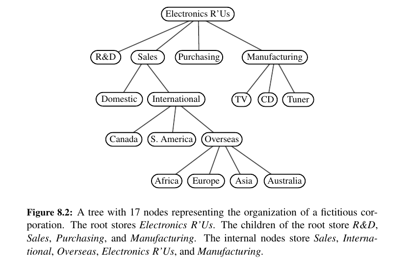
For example, the tree of Figure 8.2 has height 4. In addition, height can also be viewed as follows.
• The height of a nonempty tree T is equal to the maximum of the depths of its leaf positions.
Here is an approach for out trees, to get an idea:
def _height2(self, p):
# time is linear in size of subtree
"""Return the height of the subtree rooted at Position p."""
if self.is_leaf(p):
return 0
else:
return 1 + max(self._height2(c) for c in self.children(p))
The ability to compute heights of sub trees is beneficial, but a user might expect to be able to compute the height of the entire tree without explicitly designating the tree root.
def height(self, p = None):
"""Return the height of the subtree rooted at Position p.
If p is None, return the height of the entire tree.
"""
if p is None:
p = self.root()
return self._height2(p) # start height2 recursion
Binary Trees 🧠
In binary trees, there are 2 children for every node at most, Left or Right child.
A binary tree is an ordered tree with the following properties:
-
Every node has at most two children.
-
Each child node is labeled as being either a left child or a right child.
-
A left child precedes a right child in the order of children of a node.
The subtree rooted at a left or right child of an internal node v is called a left subtree or right subtree, respectively, of v.
A binary tree is proper if each node has either zero or two children. Some people also refer to such trees as being full binary trees.
Thus, in a proper binary tree, every internal node has exactly two children.
A binary tree that is not proper is improper.
Tip
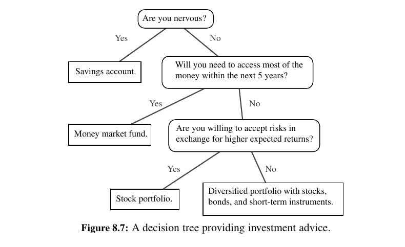
Decision Trees
An important class of binary trees arises in contexts where we wish to represent a number of different outcomes that can result from answering a series of yes-or-no questions. Each internal node is associated with a question.
Starting at the root, we go to the left or right child of the current node, depending on whether the answer to the question is “Yes” or “No.” With each decision, we follow an edge from a parent to a child, eventually tracing a path in the tree from the root to a leaf.
Such binary trees are known as decision trees, because a leaf position p in such a tree represents a decision of what to do if the questions associated with p’s ancestors are answered in a way that leads to p.
A decision tree is a proper binary tree.
An arithmetic expression can be represented by a binary tree whose leaves are associated with variables or constants, and whose internal nodes are associated with one of the operators +, −, × , and /.
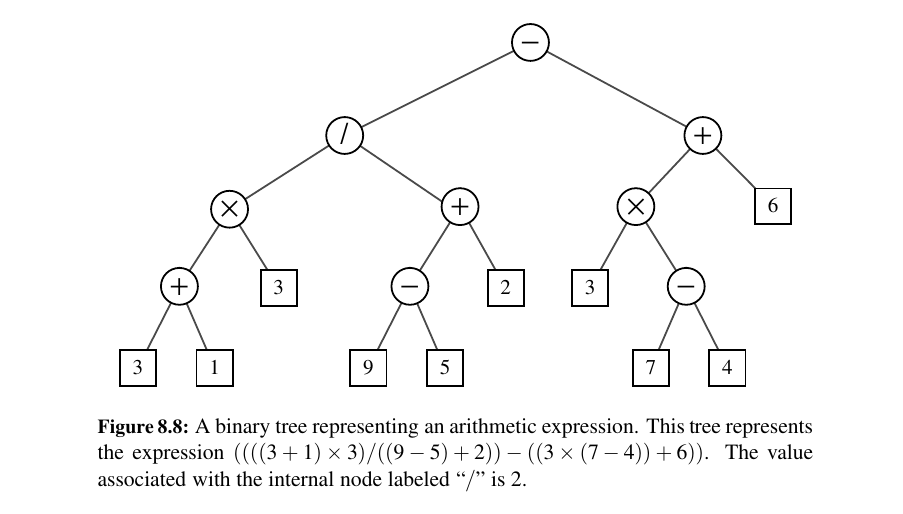
An arithmetic expression tree is a proper binary tree, since each operator +, −, ×, and / takes exactly two operands.
The Binary Tree Abstract Data Type
As an abstract data type, a binary tree is a specialization of a tree that supports three additional accessor methods:
| Method | Explained |
|---|---|
T.left(p) |
Return the position that represents the left child of p, or None if p has no left child. |
T.right(p) |
Return the position that represents the right child of p, or None if p has no right child. |
T.sibling(p) |
Return the position that represents the sibling of p, or None if p has no sibling. |
Just as Tree was defined as an abstract base class, we define a new BinaryTree class associated with the binary tree ADT. We rely on inheritance to define the BinaryTree class based upon the existing Tree class.
However, our BinaryTree class remains abstract, as we still do not provide complete specifications for how such a structure will be represented internally, nor implementations for some necessary behaviors.
By using inheritance, a binary tree supports all the functionality that was defined for general trees (e.g., parent, is_leaf, root).
Properties of Binary Trees 😍
Binary trees have several interesting properties dealing with relationships between their heights and number of nodes.
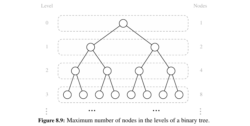
We denote the set of all nodes of a tree T at the same depth \(d\) as level d of T.
In a binary tree, level \(0\) has at most one node (the root), level \(1\) has at most two nodes (the children of the root), level \(2\) has at most four nodes, and so on (See Figure 8.9.).
In general, level \(d\) has at most \(2^d\) nodes.
In a nonempty proper binary tree T , with \(n_E\) external nodes and \(n_I\) internal nodes, we have \(n_E = n_I + 1\).
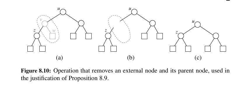
At the start, we have 5 external and 4 internal. In the end, we have 4 external and 3 internal.
Implementing Trees 🥰
The Tree and BinaryTree classes that we have defined thus far in this chapter are both formally abstract base classes.
Although they provide a great deal of support, neither of them can be directly instantiated. 😕
There are several choices for the internal representation of trees.
We describe the most common representations in this section. We begin with the case of a binary tree, since its shape is more narrowly defined.
Linked Structure for Binary Trees
A natural way to realize a binary tree T is to use a linked structure, with a node that maintains references to the element stored at a position p and to the nodes associated with the children and parent of p.
If p is the root of T , then the parent field of p is None. Likewise, if p does not have a left child (respectively, right child), the associated field is None.
The tree itself maintains an instance variable storing a reference to the root node (if any), and a variable, called size, that represents the overall number of nodes of T.
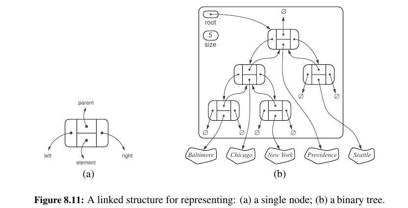
For the implementation, we define a simple, nonpublic Node class to represent a node, and a public Position class that wraps a node.
We provide a validate utility for robustly checking the validity of a given position instance when unwrapping it, and a make position utility for wrapping a node as a position to return to a caller.
For linked binary trees, a reasonable set of update methods to support for general usage are the following:
T.add_root(e): Create a root for an empty tree, storing e as the element, and return the position of that root; an error occurs if the tree is not empty.
T.add_left(p, e): Create a new node storing element e, link the node as the left child of position p, and return the resulting position; an error occurs if p already has a left child.
T.add_right(p, e): Create a new node storing element e, link the node as the right child of position p, and return the resulting position; an error occurs if p already has a right child.
T.replace(p, e): Replace the element stored at position p with element e, and return the previously stored element.
T.delete(p): Remove the node at position p, replacing it with its child, if any, and return the element that had been stored at p; an error occurs if p has two children.
T.attach(p, T1, T2): Attach the internal structure of trees T1 and T2, respectively, as the left and right sub trees of leaf position p of T, and reset T1 and T2 to empty trees; an error condition occurs if p is not a leaf.
We have specifically chosen this collection of operations because each can be implemented in \(O(1)\) worst-case time with our linked representation.
This is going to be a long one. Get ready. Here is the code:
| linked_binary_tree.py | |
|---|---|
1 2 3 4 5 6 7 8 9 10 11 12 13 14 15 16 17 18 19 20 21 22 23 24 25 26 27 28 29 30 31 32 33 34 35 36 37 38 39 40 41 42 43 44 45 46 47 48 49 50 51 52 53 54 55 56 57 58 59 60 61 62 63 64 65 66 67 68 69 70 71 72 73 74 75 76 77 78 79 80 81 82 83 84 85 86 87 88 89 90 91 92 93 94 95 96 97 98 99 100 101 102 103 104 105 106 107 108 109 110 111 112 113 114 115 116 117 118 119 120 121 122 123 124 125 126 127 128 129 130 131 132 133 134 135 136 137 138 139 140 141 142 143 144 145 146 147 148 149 150 151 152 153 154 155 156 157 158 159 160 161 162 163 164 165 166 167 168 169 170 171 172 173 174 175 176 177 178 179 180 181 | |
Performance of the Linked Binary Tree Implementation
Here is how they look:
| Method | Running Time |
|---|---|
len, is_empty |
\(O(1)\) |
root, parent, left, right, sibling, children, num_children |
\(O(1)\) |
is_root, is_leaf |
\(O(1)\) |
depth(p) |
\(O(d_p + 1)\) |
height |
\(O(n)\) |
add_root, add_left, add_right, replace, delete, attach |
\(O(1)\) |
Array-Based Representation of a Binary Tree 💕
An alternative representation of a binary tree T is based on a way of numbering the positions of T .
For every position p of T , let \(f(p)\) be the integer defined as follows.
• If p is the root of T , then \(f (p) = 0\).
• If p is the left child of position q, then \(f (p) = 2 f (q) + 1\).
• If p is the right child of position q, then \(f (p) = 2 f (q) + 2\).
The numbering function \(f\) is known as a level numbering of the positions in a binary tree T, for it numbers the positions on each level of T in increasing order from left to right.
Note well that the level numbering is based on potential positions within the tree, not actual positions of a given tree, so they are not necessarily consecutive.
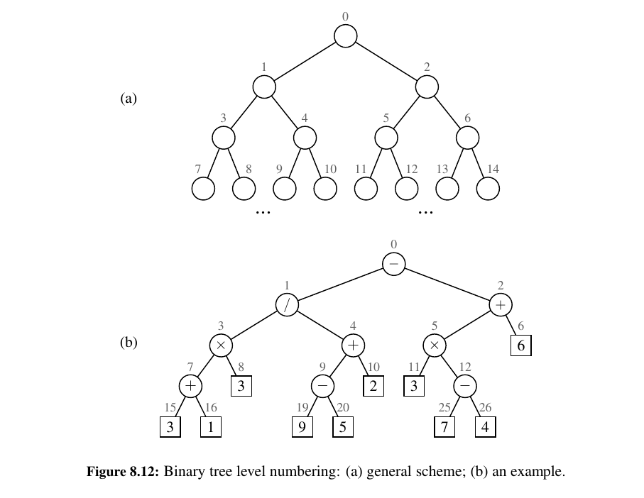
The level numbering function f suggests a representation of a binary tree T by means of an array-based structure A (such as a Python list), with the element at position p of T stored at index \(f (p)\) of the array.
One advantage of an array-based representation of a binary tree is that a position p can be represented by the single integer \(f(p)\), and that position-based methods such as root, parent, left, and right can be implemented using simple arithmetic operations on the number \(f(p)\).
Based on our formula for the level numbering, the left child of p has index \(2 f(p) + 1\), the right child of p has index \(2 f (p) + 2\), and the parent of p has index \(⌊(f (p) − 1)/2⌋\).
Tip
Here is a reminder. The notation ⌈x⌉ represents the ceiling of x, the smallest integer greater than or equal to x. The notation ⌊x⌋ represents is the floor of x, the largest integer less than or equal to x.
The space usage of an array-based representation depends greatly on the shape of the tree.
Let \(n\) be the number of nodes of T , and let \(f_M\) be the maximum value of \(f(p)\) over all the nodes of T.
The array A requires length \(N = 1 + f_M\) , since elements range from \(A[0]\) to \(A[f_M]\). Note that A may have a number of empty cells that do not refer to existing nodes of T.
In fact, in the worst case, \(N = 2^n − 1\). (Half of it is empty!)
In Chapter 9, we will see a class of binary trees, called “heaps” for which \(N = n\).
Thus, in spite of the worst-case space usage, there are applications for which the array representation of a binary tree is space efficient.
Still, for general binary trees, the exponential worst-case space requirement of this representation is prohibitive.
Another drawback of an array representation is that some update operations for trees cannot be efficiently supported. For example, deleting a node and promoting its child takes \(O(n)\) time because it is not just the child that moves locations within the array, but all descendants of that child.
Linked Structure for General Trees 😎
When representing a binary tree with a linked structure, each node explicitly maintains fields left and right as references to individual children. For a general tree, there is no a priori limit on the number of children that a node may have:
Here are the performances of the implementation of the general tree using a linked structure:
| Operation | Running Time |
|---|---|
len, is_empty |
O(1) |
root, parent, is_root, is_leaf |
O(1) |
children(p) |
\(O(c_p + 1)\) |
depth(p) |
\(O(d_p + 1)\) |
height |
\(O(n)\) |
Tree Traversal Algorithms
A traversal of a tree T is a systematic way of accessing, or “visiting” all the positions of T. A lot of ways to traverse:
Preorder and Postorder Traversals of General Trees
Preorder Traversal - Reading a World Class Book 😉 (DFS)
Tip
Here is a way to remember what preorder traversal mean: You preorder a book - you are curious - you read it all.
In a preorder traversal of a tree T , the root of T is visited first and then the sub trees rooted at its children are traversed recursively. If the tree is ordered, then the subtrees are traversed according to the order of the children.
Here is DFS in the wild:
Given the root of a binary search tree, and an integer k, return the kth
smallest value (1-indexed) of all the values of the nodes in the tree.

**Input:** root = [3,1,4,null,2], k = 1
**Output:** 1

**Input:** root = [5,3,6,2,4,null,null,1], k = 3
**Output:** 3

**Constraints:**

- The number of nodes in the tree is `n`.
- `1 <= k <= n <= 104`
- `0 <= Node.val <= 104`
Solution:
# Definition for a binary tree node.
class TreeNode:
    def __init__(self, val=0, left=None, right=None):
        self.val = val
        self.left = left
        self.right = right

class Solution:
    def kthSmallest(self, root: Optional[TreeNode], k: int) -> int:

        temp = []

        def dfs(root):
            if not root:
                return
            # go to left subtree until we find a single node
            dfs(root.left)
            if len(temp) == k:
                return
            temp.append(root.val)
            dfs(root.right)

        dfs(root)

        # last element of temp is the node we want
        return temp[-1]
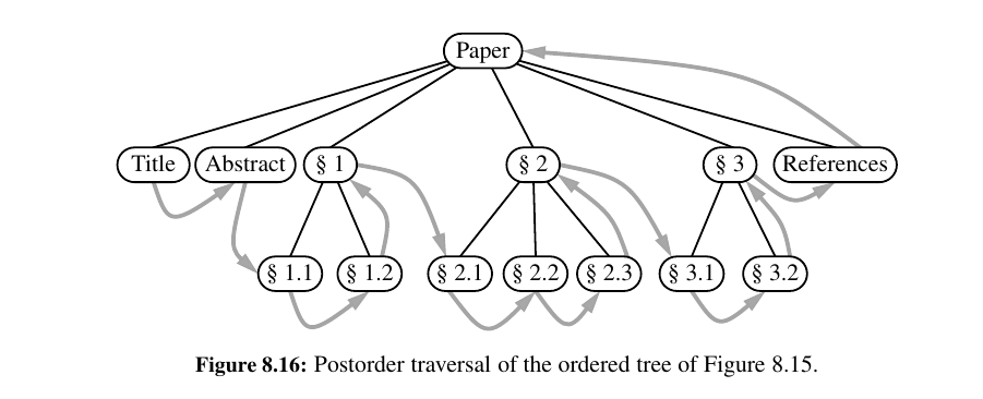
Postorder Traversal - See the Children Than Look at Parents (DFS)
Tip
Here is how you can remember what postorder traversal means. You just don't care about the noise. You just want to get to the details as soon as possible. You go deep as much as you can.
In some sense, this algorithm can be viewed as the opposite of the preorder traversal, because it recursively traverses the subtrees rooted at the children of the root first, and then visits the root (hence, the name “postorder”).
Running-Time Analysis
Both preorder and postorder traversal algorithms are efficient ways to access all the positions of a tree.
The overall running time for the traversal of tree T is \(O(n)\), where \(n\) is the number of positions in the tree. This running time is asymptotically optimal since the traversal must visit all the \(n\) positions of the tree.
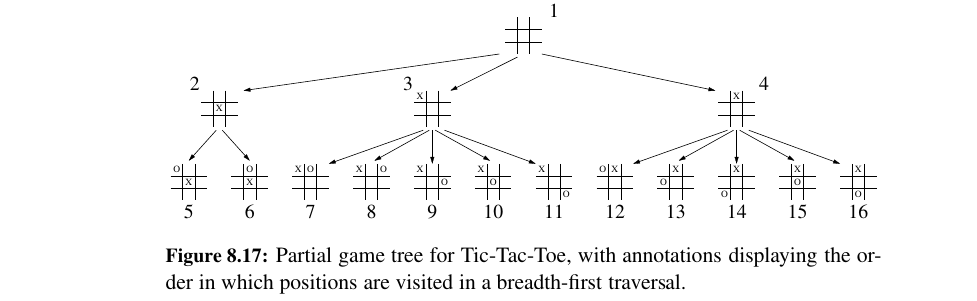
Breadth-First Tree Traversal
Tip
Breadth-First Search - BFS -> See Everyone At This Level Than Go Deeper 😍
Another common approach is to traverse a tree so that we visit all the positions at depth d before we visit the positions at depth d + 1. Such an algorithm is known as a breadth-first traversal.
Inorder Traversal of a Binary Tree
Tip
Inorder Traversal -> Swipe from Left -> Right (DFS)
During an inorder traversal, we visit a position between the recursive traversals of its left and right subtrees.
The inorder traversal of a binary tree T can be informally viewed as visiting the nodes of T “from left to right.”
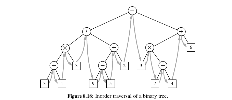
3 + 1 × 3/9 − 5 + 2 ...
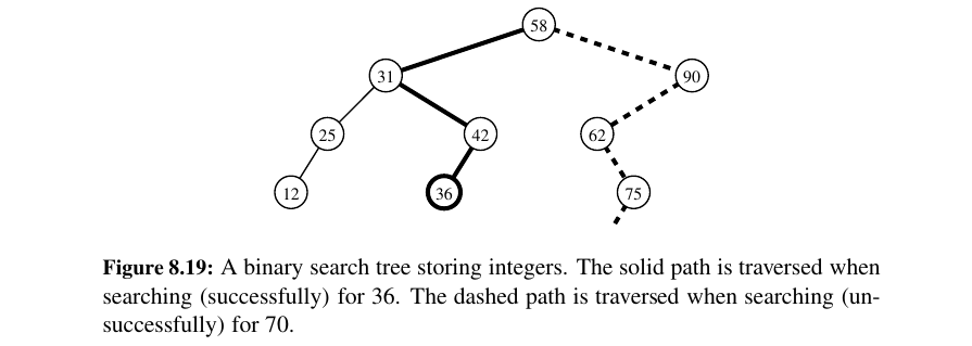
Binary Search Trees 🤔
An important application of the inorder traversal algorithm arises when we store an ordered sequence of elements in a binary tree, defining a structure we call a binary search tree.
Let S be a set whose unique elements have an order relation.
For example, S could be a set of integers.
A binary search tree for S is a binary tree T such that, for each position p of T :
• Position p stores an element of S, denoted as e(p).
• Elements stored in the left subtree of p (if any) are less than e(p).
• Elements stored in the right subtree of p (if any) are greater than e(p).
A binary search tree can be viewed as a binary decision tree (recall Example 8.6), where the question asked at each internal node is whether the element at that node is less than, equal to, or larger than the element being searched for.
Chapter 11 is devoted to the study of search trees.
Implementing Tree Traversals in Python
When first defining the tree ADT in Chapter 8.1.2, we stated that tree T should include support for the following methods:
• T.positions(): Generate an iteration of all positions of tree T.
• iter(T): Generate an iteration of all elements stored within tree T.
At that time, we did not make any assumption about the order in which these iterations report their results.
In this section, we demonstrate how any of the tree traversal algorithms we have introduced could be used to produce these iterations.
Preorder Traversal
Formally, both preorder and the utility _subtree_preorder are generators.
Rather than perform a “visit” action from within this code, we yield each position to the caller and let the caller decide what action to perform at that position.
def preorder(self):
    """Generate a preorder iteration of positions in the tree."""
    if not self.is_empty():
        for p in self._subtree_preorder(self.root()): # start recursion
            yield p

def _subtree_preorder(self, p):
    """Generate a preorder iteration of positions in subtree rooted at p."""
    yield p # visit p before its subtrees
    for c in self.children(p): # for each child c
        for other in self._subtree_preorder(c): # do preorder of c’s subtree
            yield other # yielding each to our caller
Postorder Traversal
We can implement a postorder traversal using very similar technique as with a preorder traversal.
The only difference is that within the recursive utility for a post-order we wait to yield position p until after we have recursively yield the positions in its subtrees.
Children before parents!
def postorder(self):
    """Generate a postorder iteration of positions in the tree."""
    if not self.is_empty( ):
        for p in self._subtree_postorder(self.root( )): # start recursion
            yield p

def _subtree_postorder(self, p):
    """Generate a postorder iteration of positions in subtree rooted at p."""
    for c in self.children(p): # for each child c
        for other in self._subtree_postorder(c): # do postorder of c’s subtree
            yield other   # yielding each to our caller
    yield p # visit p after its subtrees
Breadth First Traversal
We can use a Queue (A LinkedQueue) for this solution. Add the level to the root, and as you empty it add the children of those nodes in the current level.
def breadthfirst(self):
    """Generate a breadth-first iteration of the positions of the tree."""
    if not self.is_empty():
        fringe = LinkedQueue() # known positions not yet yielded
        fringe.enqueue(self.root()) # starting with the root
        while not fringe.is_empty():
            p = fringe.dequeue( ) # remove from front of the queue
            yield p # report this position
            for c in self.children(p):
                fringe.enqueue(c) # add children to back of queue
Inorder Traversal
The idea is cool here. You traverse the left tree, you travel the parent than you travel the right tree.
def inorder(self):
    """Generate an inorder iteration of positions in the tree."""
    if not self.is_empty():
        for p in self._subtree_inorder(self.root()):
            yield p

def _subtree_inorder(self, p):
    """Generate an inorder iteration of positions in subtree rooted at p."""
    if self.left(p) is not None:  # if left child exists, traverse its subtree
        for other in self._subtree_inorder(self.left(p)):
            yield other

    yield p  # visit p between its subtrees

    if self.right(p) is not None:  # if right child exists, traverse its subtree
        for other in self._subtree_inorder(self.right(p)):
            yield other
Applications of Tree Traversals
Wisdom: Here is my way to remember the traversals: Reading a book is preorder, filesystem is postorder, swipe from left to right is inorder.
Here are some examples for using the tree traversals we learned.
Table of Contents
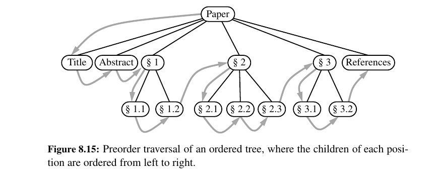
When using a tree to represent the hierarchical structure of a document, a preorder traversal of the tree can naturally be used to produce a table of contents for the document.
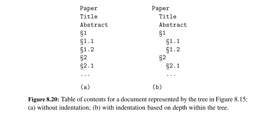
We indent each element with a number of spaces equal to twice the element’s depth in the tree
def preorder_label(T, p, d, path):
    """Print labeled representation of subtree of T rooted at p at depth d."""
    label = ".".join(str(j+1) for j in path) # displayed labels are one-indexed
    print(2 * d * " " + label, p.element())
    path.append(0) # path entries are zero-indexed
    for c in T.children(p):
        preorder_label(T, c, d+1, path) # child depth is d+1
        path[−1] += 1
    path.pop()
Parenthetic Representations of a Tree
It is not possible to reconstruct a general tree, given only the preorder sequence of elements.
Some additional context is necessary for the structure of the tree to be well defined. The use of indentation or numbered labels provides such context, with a very human-friendly presentation.
However, there are more concise string representations of trees that are computer-friendly.
is where p is the root of T and \(T_1\), \(T_2\), . . . , \(T_k\) are the subtrees rooted at the children of p, which are given in order if T is an ordered tree.
The opening parenthesis must be produced just before the loop over a position’s children and the closing parenthesis must be produced just after that loop:
def parenthesize(T, p):
    """Print parenthesized representation of subtree of T rooted at p."""
    print(p.element(), end='' )  # use of end avoids trailing newline
    if not T.is_leaf(p):
        first time = True
        for c in T.children(p):
            sep = ' (' if first time else ', '  # determine proper separator
            print(sep, end='')
            first time = False # any future passes will not be the first
            parenthesize(T, c)   # recur on child
        print(")" , end='') # include closing parenthesis
Computing Disk Space
The recursive computation of disk space is emblematic of a postorder traversal, as we cannot effectively compute the total space used by a directory until after we know the space that is used by its children directories.
def disk_space(T, p):
    """Return total disk space for subtree of T rooted at p."""
    subtotal = p.element().space()  # space used at position p
    for c in T.children(p):
        subtotal += disk space(T, c)  # add child’s space to subtotal
    return subtotal
Euler Tours and the Template Method Pattern 🤔
Unfortunately, they also show that the specific implementations of the preorder and postorder methods of our Tree class, or the inorder method of the BinaryTree class, are not general enough to capture the range of computations we desire.
In some cases, we need more of a blending of the approaches, with initial work performed before recurring on subtrees, additional work performed after those recursions, and in the case of a binary tree, work performed between the two possible recursions.
Furthermore, in some contexts it was important to know the depth of a position, or the complete path from the root to that position, or to return information from one level of the recursion to another.
In this section, we develop a more general framework for implementing tree traversals based on a concept known as an Euler Tour traversal.
The Euler Tour traversal of a general tree T can be informally defined as a “walk” around T, where we start by going from the root toward its leftmost child, viewing the edges of T as being “walls” that we always keep to our left.
Tip
Euler Tour: We walk around hugging an invisible walk around tree.
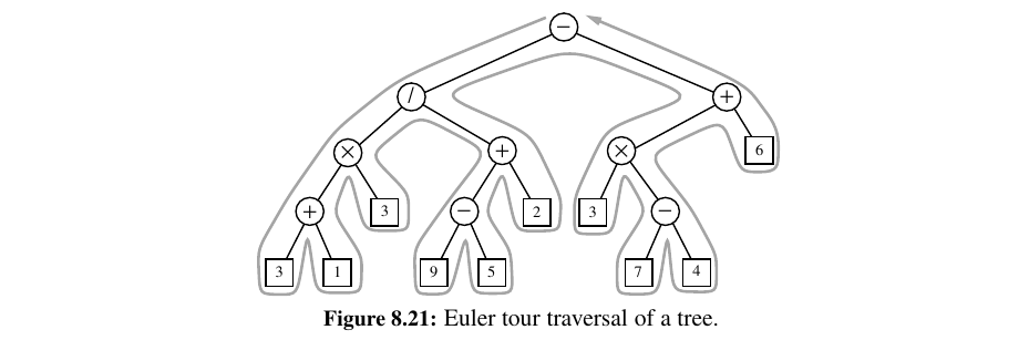
The complexity of the walk is \(O(n)\), because it progresses exactly two times along each of the \(n−1\) edges of the tree—once going downward along the edge, and later going upward along the edge.
Here is the code:
Formally, our framework relies on the following two hooks that can be specialized:
• _hook_previsit(p, d, path): This function is called once for each position, immediately before its subtrees (if any) are traversed. Parameter p is a position in the tree, d is the depth of that position, and path is a list of indices, using the convention described in the discussion of Code Fragment 8.24. No return value is expected from this function.
• _hook_postvisit(p, d, path, results): This function is called once for each position, immediately after its subtrees (if any) are traversed. The first three parameters use the same convention as did hook previsit. The final parameter is a list of objects that were provided as return values from the post visits of the respective subtrees of p. Any value returned by this call will be available to the parent of p during its postvisit.
Using Euler Tour
Here is a simplification for the indented printing with numbers problem:
class PreorderPrintIndentedLabeledTour(EulerTour):
    def _hook_previsit(self, p, d, path):
        label = ".".join(str(j+1) for j in path) # labels are one-indexed
        print(2 * d * " " + label, p.element())
Or disk space problem:
class DiskSpaceTour(EulerTour):
    def _hook_postvisit(self, p, d, path, results):
        # we simply add space associated with p to that of its subtrees
        return p.element().space() + sum(results)
The Euler Tour Traversal of a Binary Tree
We introduced the concept of an Euler Tour traversal of a general graph, using the template method pattern in designing the EulerTour class.
That class provided methods hook previsit and hook postvisit that could be overridden to customize a tour.
Down below we provide a BinaryEulerTour specialization that includes an additional hook invisit that is called once for each position—after its left subtree is traversed, but before its right subtree is traversed.
We can use this class when we want to draw a graphical layout for a tree:
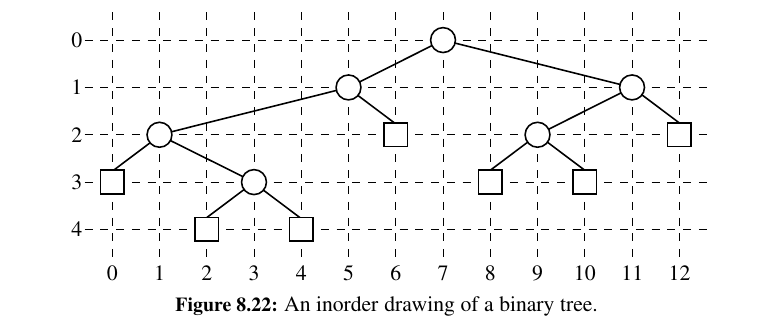
The geometry is determined by an algorithm that assigns x- and y-coordinates to each position p of a binary tree T using the following two rules:
• x(p) is the number of positions visited before p in an inorder traversal of T .
• y(p) is the depth of p in T .
In this application, we take the convention common in computer graphics that x - coordinates increase left to right and y - coordinates increase top to bottom. So the origin is in the upper left corner of the computer screen.
class BinaryLayout(BinaryEulerTour):
    """Class for computing (x,y) coordinates for each node of a binary tree."""

    def __init__(self, tree):
        super().__init__(tree)  # must call the parent constructor
        self._count = 0  # initialize count of processed nodes

    def _hook_invisit(self, p, d, path):
        p.element().setX(self._count)  # x-coordinate serialized by count
        p.element().setY(d)  # y-coordinate is depth
        self._count += 1  # advance count of processed nodes
Case Study: An Expression Tree
In this section, we define a new ExpressionTree class that provides support for constructing such trees, and for displaying and evaluating the arithmetic expression that such a tree represents.
Our ExpressionTree class is defined as a subclass of LinkedBinaryTree, and we rely on the nonpublic mutators to construct such trees.
Each internal node must store a string that defines a binary operator (e.g., + ), and each leaf must store a numeric value (or a string representing a numeric value).
Our eventual goal is to build arbitrarily complex expression trees for compound arithmetic expressions such as \((((3 + 1) × 4)/((9 − 5) + 2))\).
Using a stack, we can build an expression tree:
def build_expression_tree(tokens):
    """Returns an ExpressionTree based upon by a tokenized expression.
    tokens must be an iterable of strings representing a fully parenthesized
    binary expression, such as ['(', '43', '-', '(', '3', '*', '10', ')', ')']
    """
    S = []  # we use Python list as stack
    for t in tokens:
        if t in '+-x*/':  # t is an operator symbol
            S.append(t)  # push the operator symbol
        elif t not in '()':  # consider t to be a literal
            S.append(ExpressionTree(t))  # push trivial tree storing value
        elif t == ')':  # compose a new tree from three constituent parts
            right = S.pop()  # right subtree as per LIFO
            op = S.pop()  # operator symbol
            left = S.pop()  # left subtree
            S.append(ExpressionTree(op, left, right))  # repush tree
            # we ignore a left parenthesis
    return S.pop()
You are doing incredible. Let's now move on to priority queues and explore more! 🐤