Search Trees
Binary Search Trees 😍
Tip
Binary search trees are well-suited for implementing sorted maps, as they maintain key-value pairs in order.
Binary Search Trees (BSTs) exist as a data structure because they provide an efficient way to organize and search for data.
The primary purpose of a Binary Search Tree is to support fast search, insertion, and deletion of elements in a sorted order.
To be precise, binary search trees provide an average Big-O complexity of \(O(log(n))\) for search, insert, update, and delete operations. \(log(n)\) is much faster than the linear \(O(n)\) time required to find elements in an unsorted array. Many popular production databases such as PostgreSQL and MySQL use binary trees under the hood to speed up CRUD operations.
Pros of Binary Search Trees
- When balanced, a BST provides lightning-fast
O(log(n))insertions, deletions, and lookups.- Binary search trees are simple to implement. An ordinary BST, unlike a balanced red-black tree, requires very little code to get running.
Cons of Binary Search Trees
- Slow for a brute-force search. If you need to iterate over each node, you might have more success with an array.
- When the tree becomes unbalanced, all fast
O(log(n))operations quickly degrade toO(n).- Since pointers to whole objects are typically involved, a BST can require quite a bit more memory than an array, although this depends on the implementation.
In Chapter 8 we introduced the tree data structure and demonstrated a variety of applications. One important use is as a search tree.
In this chapter, we use a search tree structure to efficiently implement a sorted map.
The three most fundamental methods of a map M are __getitem__, __setitem__ and __delitem__ 😍
-
M[k]: Return the value v associated with key k in map M, if one exists; otherwise raise aKeyError; implemented with__getitem__method. -
M[k] = v: Associate value v with key k in map M, replacing the existing value if the map already contains an item with key equal to k; implemented with__setitem__method. -
del M[k]: Remove from map M the item with key equal to k; if M has no such item, then raise aKeyError; implemented with__delitem__method.
The sorted map ADT includes additional functionality (see Chapter 10.3), guaranteeing that an iteration reports keys in sorted order, and supporting additional searches such as find_gt(k) and find_range(start, stop).
Binary trees are an excellent data structure for storing items of a map, assuming we have an order relation defined on the keys.
In this context, a binary search tree is a binary tree T with each position p storing a key-value pair (k, v) such that:
• Keys stored in the left subtree of p are less than k.
• Keys stored in the right subtree of p are greater than k.
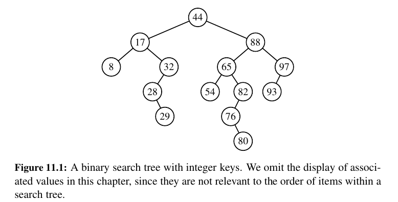
Left is less than root, right is more than root!
Navigating a Binary Search Tree 💚
An inorder traversal of a binary search tree visits positions in increasing order of their keys.
Since an inorder traversal can be executed in linear time, a consequence of this proposition is that we can produce a sorted iteration of the keys of a map in linear time, when represented as a binary search tree.
Searches 😍
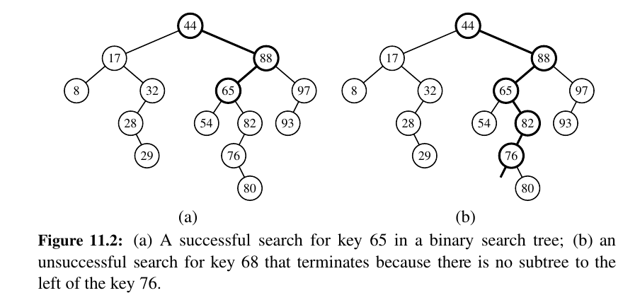
The most important consequence of the structural property of a binary search tree is its namesake search algorithm.
We can attempt to locate a particular key in a binary search tree by viewing it as a decision tree (recall Figure 8.7).
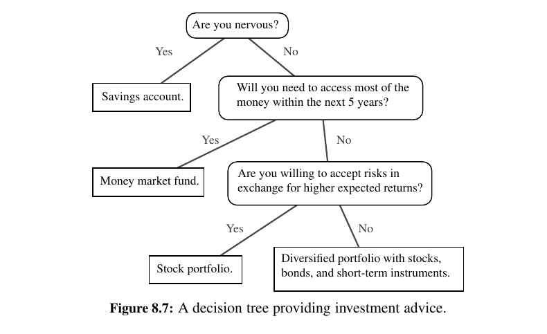
In this case, the question asked at each position p is whether the desired key k is less than, equal to, or greater than the key stored at position p, which we denote as p.key().
If the answer is “less than,” then the search continues in the left subtree.
If the answer is “equal,” then the search terminates successfully. If the answer is “greater than,” then the search continues in the right subtree.
Finally, if we reach an empty subtree, then the search terminates unsuccessfully.
We spend \(O(1)\) time per position encountered in the search, the overall search runs in \(O(h)\) time, where h is the height of the binary search tree T.
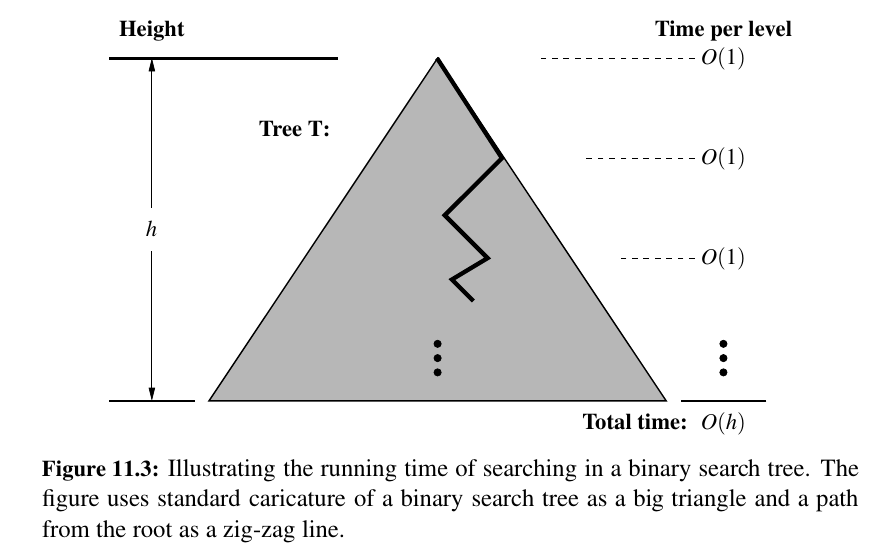
Admittedly, the height \(h\) of T can be as large as the number of entries, \(n\), but we expect that it is usually much smaller.
Indeed, later in this chapter we show various strategies to maintain an upper bound of \(O(log n)\) on the height of a search tree T.
Insertions and Deletions
Insertion:
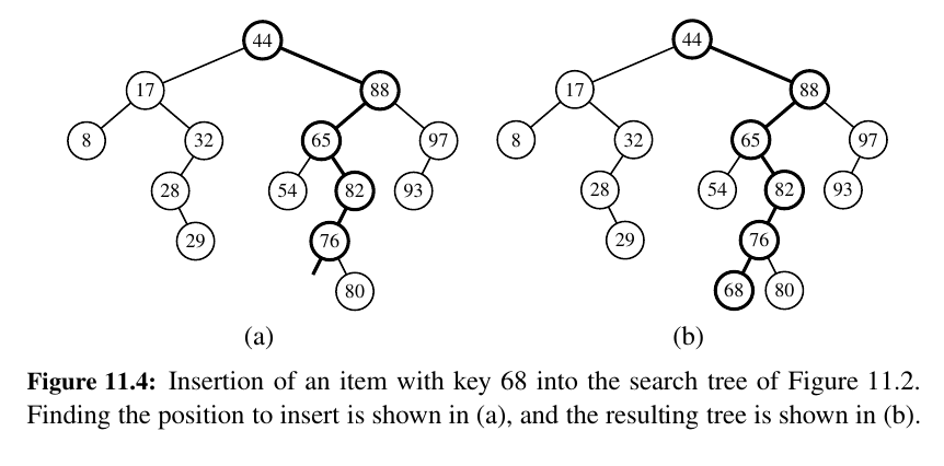
We begin with a search for key k (assuming the map is nonempty).
If found, that item’s existing value is reassigned.
Otherwise, a node for the new item can be inserted into the underlying tree T in place of the empty subtree that was reached at the end of the failed search.
Algorithm TreeInsert(T, k, v):
    Input: A search key k to be associated with value v
    p = TreeSearch(T, T.root(), k)
    if k == p.key() then
        Set p’s value to v
    else if k < p.key() then
        add node with item (k,v) as left child of p
    else
        add node with item (k,v) as right child of p
Deletion
Deleting an item from a binary search tree T is a bit more complex than inserting a new item because the location of the deletion might be anywhere in the tree. (In contrast, insertions are always enacted at the bottom of a path.)
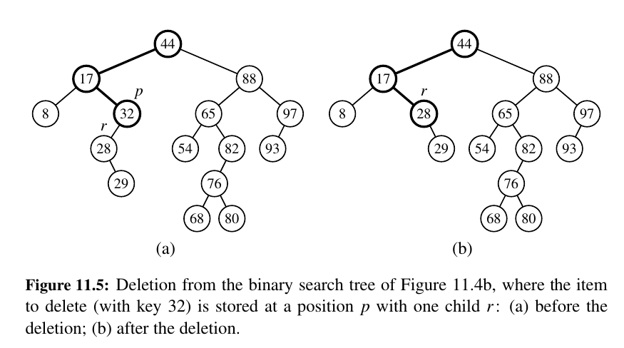
Start searching for the node you want to delete. If the search is successful, we distinguish between two cases:
If only one child - Remove and Replace!
1) It removes the item with key k from the map while maintaining all other ancestor-descendant relationships in the tree, thereby assuring the upkeep of the binary search tree property.
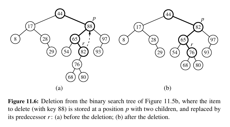
If two children, find before, use it as replacement, delete!
2) If position p has two children, we cannot simply remove the node from T since this would create a “hole” and two orphaned children.
Python Implementation
With a multiple inheritance, here is the code:
| tree_map.py | |
|---|---|
1 2 3 4 5 6 7 8 9 10 11 12 13 14 15 16 17 18 19 20 21 22 23 24 25 26 27 28 29 30 31 32 33 34 35 36 37 38 39 40 41 42 43 44 45 46 47 48 49 50 51 52 53 54 55 56 57 58 59 60 61 62 63 64 65 66 67 68 69 70 71 72 73 74 75 76 77 78 79 80 81 82 83 84 85 86 87 88 89 90 91 92 93 94 95 96 97 98 99 100 101 102 103 104 105 106 107 108 109 110 111 112 113 114 115 116 117 118 119 120 121 122 123 124 125 126 127 128 129 130 131 132 133 134 135 136 137 138 139 140 141 142 143 144 145 146 147 148 149 150 151 152 153 154 155 156 157 158 159 160 161 162 163 164 165 166 167 168 169 170 171 172 173 174 175 176 177 178 179 180 181 182 183 184 185 186 187 188 189 190 191 192 193 194 195 196 197 198 199 200 201 202 203 204 205 206 207 208 209 210 211 212 213 214 215 216 217 218 219 220 221 222 223 224 225 226 227 228 229 230 231 232 233 234 235 236 237 238 239 240 241 242 | |
...
Performance of a Binary Search Tree
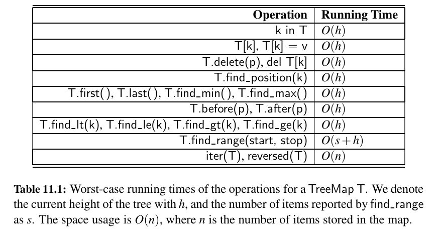
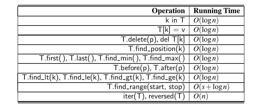
An analysis of the operations of our TreeMap class is given in Table 11.1.
Almost all operations have a worst-case running time that depends on \(h\), where \(h\) is the height of the current tree.
This is because most operations rely on a constant amount of work for each node along a particular path of the tree, and the maximum path length within a tree is proportional to the height of the tree.
IMPORTANT 😦
Warning
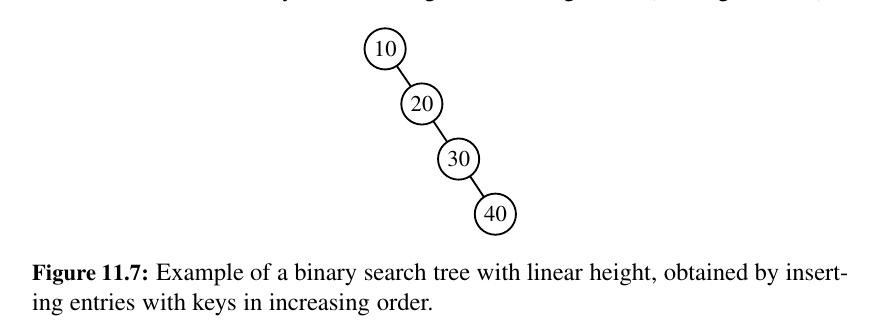
If you insert keys in strictly increasing or decreasing order, a basic binary search tree becomes completely unbalanced — essentially turning into a linked list!
A binary search tree T is therefore an efficient implementation of a map with n entries only if its height is small.
In the best case, T has height \(h = ⌈log(n+ 1)⌉ − 1\), which yields logarithmic-time performance for all the map operations.
In the worst case, however, T has height \(n\), in which case it would look and feel like an ordered list implementation of a map.
Such a worst-case configuration arises, for example, if we insert items with keys in increasing or decreasing order. (See Figure 11.7.)
In applications where one cannot guarantee the random nature of updates, it is better to rely on variations of search trees, presented in the remainder of this chapter, that guarantee a worst-case height of \(O(log(n)),\) and thus \(O(log(n))\) worst-case time for searches, insertions, and deletions.
Balanced Search Trees 😍
In the closing of the previous section, we noted that if we could assume a random series of insertions and removals, the standard binary search tree supports \(O(log n)\) expected running times for the basic map operations.
However, we may only claim \(O(n)\) worst-case time, because some sequences of operations may lead to an unbalanced tree with height proportional to n.
In the remainder of this chapter, we explore four search tree algorithms that provide stronger performance guarantees.
Three of the four data structures (AVL trees, splay trees, and red-black trees) are based on augmenting a standard binary search tree with occasional operations to reshape the tree and reduce its height.
The primary operation to rebalance a binary search tree is known as a rotation. During a rotation, we “rotate” a child to be above its parent, as diagrammed in Figure 11.8.
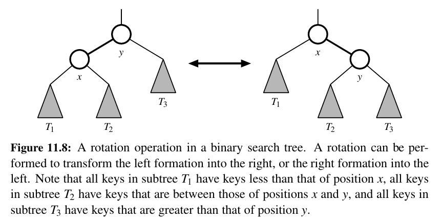
To maintain the binary search tree property through a rotation, we note that if position x was a left child of position y prior to a rotation (and therefore the key of x is less than the key of y), then y becomes the right child of x after the rotation, and vice versa.
Furthermore, we must relink the subtree of items with keys that lie between the keys of the two positions that are being rotated.
In the context of a tree-balancing algorithm, a rotation allows the shape of a tree to be modified while maintaining the search tree property.
One or more rotations can be combined to provide broader re balancing within a tree.
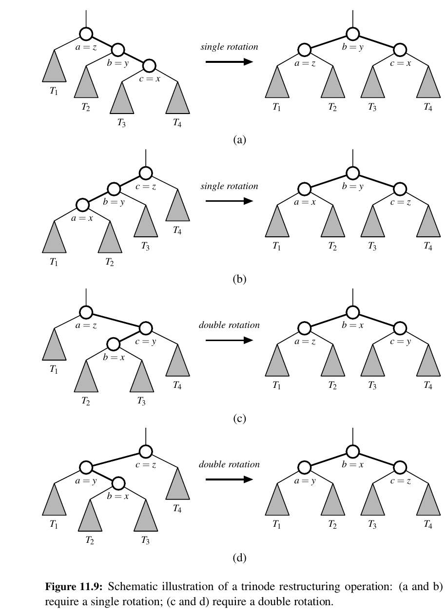
One such compound operation we consider is a trinode restructuring.
For this manipulation, we consider a position x, its parent y, and its grandparent z.
The goal is to restructure the subtree rooted at z in order to reduce the overall path length to x and its subtrees.
In practice, the modification of a tree T caused by a trinode restructuring operation can be implemented through case analysis either as a single rotation (as in Figure 11.9a and b) or as a double rotation (as in Figure 11.9c and d).
The double rotation arises when position x has the middle of the three relevant keys and is first rotated above its parent, and then above what was originally its grandparent.
In any of the cases, the trinode restructuring is completed with \(O(1)\) running time.
Python Framework for Balancing Search Trees
Our TreeMap class does not have any balancing.
It is supposed to be a base class:
Hooks for Rebalancing Operations
Our implementation of the basic map operations in Chapter 11.1.4 includes strategic calls to three nonpublic methods that serve as hooks for rebalancing algorithms:
• A call to _rebalance_insert(p) is made from within the __setitem__ method immediately after a new node is added to the tree at position p.
• A call to _rebalance_delete(p) is made each time a node has been deleted from the tree, with position p identifying the parent of the node that has just been removed. Formally, this hook is called from within the public delete(p) method, which is indirectly invoked by the public __delitem__(k) behavior.
• We also provide a hook, _rebalance_access(p), that is called when an item at position p of a tree is accessed through a public method such as __getitem__. This hook is used by the splay tree structure (see Section 11.4) to restructure a tree so that more frequently accessed items are brought closer to the root.
We provide trivial declarations of these three methods down below, having bodies that do nothing (using the pass statement).
A subclass of TreeMap may override any of these methods to implement a nontrivial action to rebalance a tree.
This is another example of the template method design pattern, as seen in Section 8.4.6.
def _rebalance_insert(self, p): pass
def _rebalance_delete(self, p): pass
def _rebalance_access(self, p): pass
Tip
The TreeMap class, which uses a standard binary search tree as its data structure, should be an efficient map data structure, but its worst-case performance for the various operations is linear time, because it is possible that a series of operations results in a tree with linear height. 💙
In this section, we describe a simple balancing strategy that guarantees worst-case logarithmic running time for all the fundamental map operations.
AVL Trees - Satisfying Height - Balance 💕
The simple correction is to add a rule to the binary search tree definition that will maintain a logarithmic height for the tree.
Although we originally defined the height of a subtree rooted at position p of a tree to be the number of edges on the longest path from p to a leaf (see Chapter 8.1.3), it is easier for explanation in this section to consider the height to be the number of nodes on such a longest path.
By this definition, a leaf position has height 1, while we trivially define the height of a “null” child to be 0.
In this section, we consider the following height-balance property, which characterizes the structure of a binary search tree T in terms of the heights of its nodes.
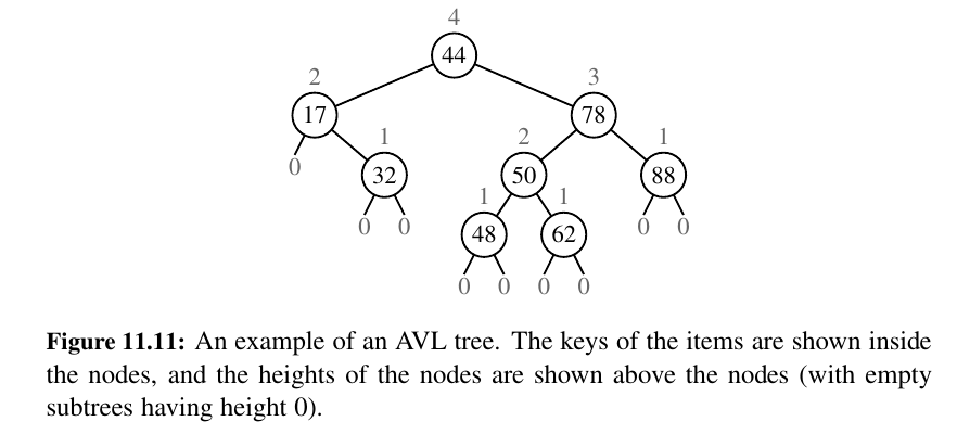
Height-Balance Property: For every position p of T , the heights of the children of p differ by at most 1.
Any binary search tree T that satisfies the height-balance property is said to be an AVL tree, named after the initials of its inventors:
An immediate consequence of the height-balance property is that a subtree of an AVL tree is itself an AVL tree. The height-balance property has also the important consequence of keeping the height small, as shown in the following proposition.
Wisdom: The height of an AVL tree storing n entries is \(O(log n)\).
Update Operations
Insertion
We have to restore balance after every insertion:
We restore the balance of the nodes in the binary search tree T by a simple “search-and-repair” strategy.
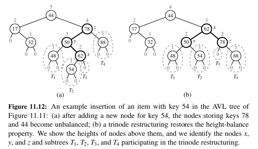
In particular, let z be the first position we encounter in going up from p toward the root of T such that z is unbalanced (see Figure 11.12a.)
Also, let y denote the child of z with higher height (and note that y must be an ancestor of p).
Finally, let x be the child of y with higher height (there cannot be a tie and position x must also be an ancestor of p, possibly p itself).
We rebalance the subtree rooted at z by calling the trinode restructuring method, restructure(x).
Deletion:
TODO
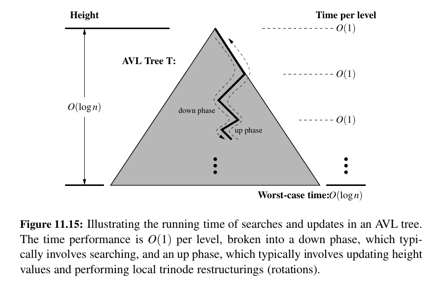
Performance of AVL Trees
By Proposition 11.2, the height of an AVL tree with n items is guaranteed to be \(O(log n)\).
Because the standard binary search tree operation had running times bounded by the height (see Table 11.1), and because the additional work in maintaining balance factors and restructuring an AVL tree can be bounded by the length of a path in the tree, the traditional map operations run in worst-case logarithmic time with an AVL tree.
...
Python Implementation
TODO: Not urgent
...
Here is the code:
Splay Trees 🏂
What are Splay Trees?
The next search tree structure we study is known as a a splay tree.
This structure is conceptually quite different from the other balanced search trees we discuss in this chapter, for a splay tree does not strictly enforce a logarithmic upper bound on the height of the tree.
In fact, there are no additional height, balance, or other auxiliary data associated with the nodes of this tree.
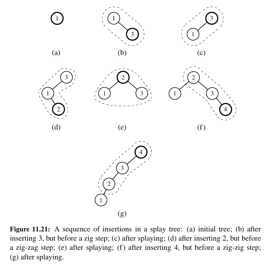
The efficiency of splay trees is due to a certain move-to-root operation, called splaying, that is performed at the bottom most position p reached during every insertion, deletion, or even a search.
In essence, this is a tree variant of the move-to-front heuristic that we explored for lists in Chapter 7.6.2.
Intuitively, a splay operation causes more frequently accessed elements to remain nearer to the root, thereby reducing the typical search times.
The surprising thing about splaying is that it allows us to guarantee a logarithmic amortized running time, for insertions, deletions, and searches.
Splaying 🏂
Given a node x of a binary search tree T , we splay x by moving x to the root of T through a sequence of restructurings.
The particular restructurings we perform are important, for it is not sufficient to move x to the root of T by just any sequence of restructurings.
The specific operation we perform to move x up depends upon the relative positions of x, its parent y, and (if it exists) x’s grandparent z.
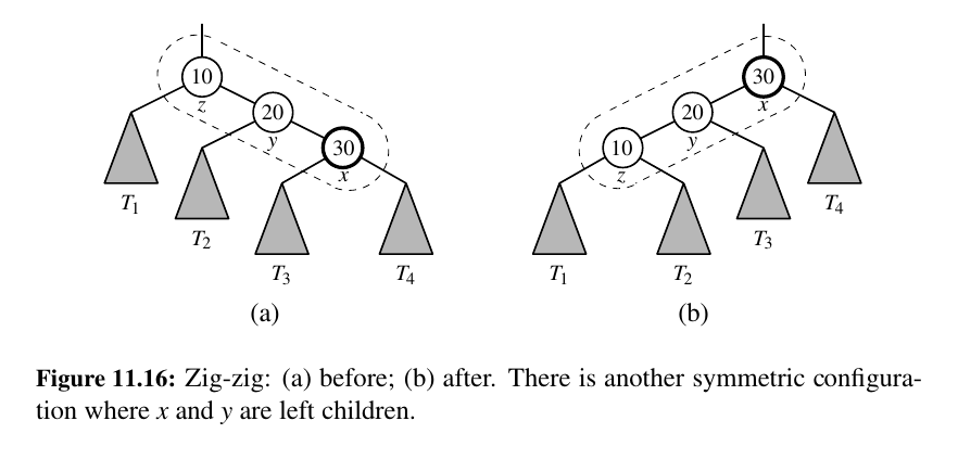
zig-zig
The node x and its parent y are both left children or both right children (See Figure 11.16).
We promote x, making y a child of x and z a child of y, while maintaining the inorder relationships of the nodes in T .
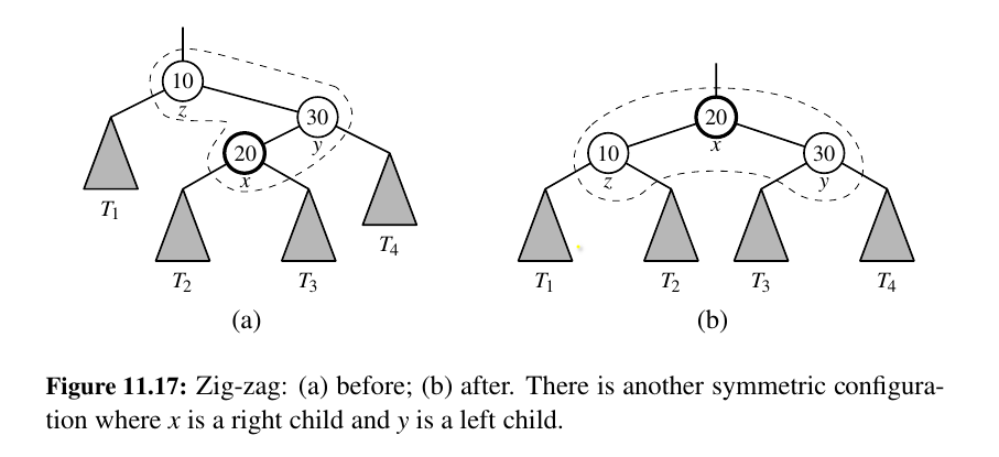
zig-zag
One of x and y is a left child and the other is a right child (See Figure 11.17).
In this case, we promote x by making x have y and z as its children, while maintaining the inorder relationships of the nodes in T .
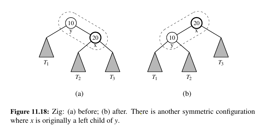
zig
x does not have a grandparent (See Figure 11.18).
In this case, we perform a single rotation to promote x over y, making y a child of x, while maintaining the relative inorder relationships of the nodes in T .
TODO: Not urgent
...
When to Splay
Just add the figures for now.
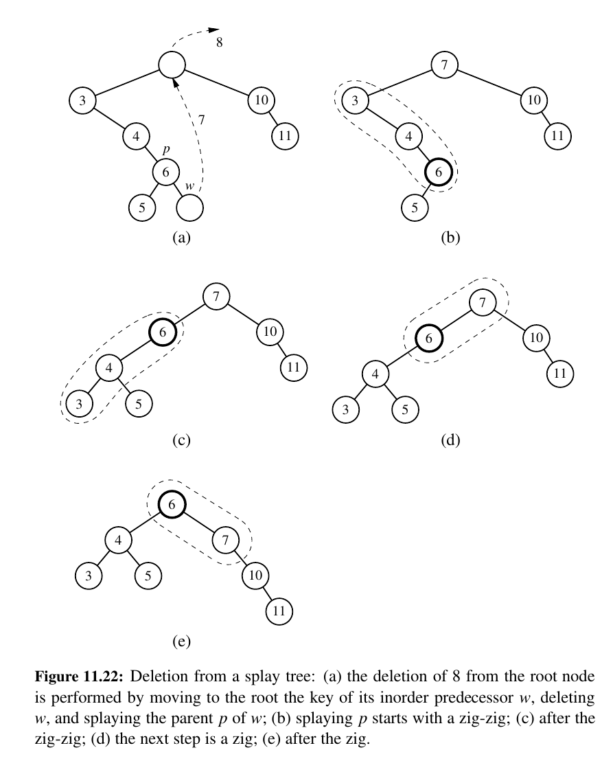
Deletion:
TODO: Not urgent
...
Python Implementation
TODO: Not urgent
...
Here is the code:
Amortized Analysis of Splaying
The time for performing a splaying step for a position p is asymptotically the same as the time needed just to reach that position in a top-down search from the root of T.
Tip
The amortized running time of performing a search, insertion, or deletion in a splay tree is O(log n), where n is the size of the splay tree at the time.
Thus, a splay tree can achieve logarithmic-time amortized performance for implementing a sorted map ADT.
This amortized performance matches the worst-case performance of AVL trees, (2, 4) trees, and red-black trees, but it does so using a simple binary tree that does not need any extra balance information stored at each of its nodes.
TODO: Not urgent
...
(2,4) Trees
What are (2,4) Trees?
(2,4) tree is a particular example of a more general structure known as a multiway search tree, in which internal nodes may have more than two children.
Other forms of multiway search trees will be discussed in Chapter 15.
Recall that general trees are defined so that internal nodes may have many children. In this section, we discuss how general trees can be used as multiway search trees.
Map items stored in a search tree are pairs of the form (k, v), where k is the key and v is the value associated with the key.
Multiway Search Trees
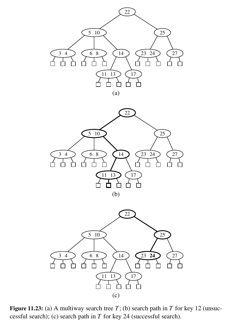
Let w be a node of an ordered tree. We say that w is a d-node if w has d children. We define a multiway search tree to be an ordered tree T that has the following properties, which are illustrated in Figure 11.23a:
• Each internal node of T has at least two children. That is, each internal node is a d-node such that \(d ≥ 2\).
• Each internal d-node w of T with children \(c_1 , . . . , c_d\) stores an ordered set of \(d − 1\) key-value pairs \((k_1 , v_1 ), . . ., (k_{d−1} , v_{d−1})\), where \(k_1 ≤ · · · ≤ k_{d−1}\) .
• Let us conventionally define \(k_0 = −∞\) and \(k_d = +∞\). For each item (k, v) stored at a node in the subtree of w rooted at \(c_i , i = 1, . . . , d\), we have that \(k_{i−1} ≤ k ≤ k_{i}\) .
That is, if we think of the set of keys stored at w as including the special fictitious keys \(k_0 = −∞\) and \(k_d = +∞\), then a key k stored in the subtree of T rooted at a child node \(c_i\) must be “in between” two keys stored at w.
This simple viewpoint gives rise to the rule that a d-node stores d − 1 regular keys, and it also forms the basis of the algorithm for searching in a multiway search tree.
By the above definition, the external nodes of a multiway search do not store any data and serve only as “placeholders.”
These external nodes can be efficiently represented by None references, as has been our convention with binary search trees (Chapter 11.1).
However, for the sake of exposition, we will discuss these as actual nodes that do not store anything.
Based on this definition, there is an interesting relationship between the number of key-value pairs and the number of external nodes in a multiway search tree.
Proposition 11.7: An n-item multiway search tree has n + 1 external nodes.
TODO: Not urgent
...
(2,4)-Tree Operations
A multiway search tree that keeps the secondary data structures stored at each node small and also keeps the primary multiway tree balanced is the (2, 4) tree, which is sometimes called a 2-4 tree or 2-3-4 tree.
This data structure achieves these goals by maintaining two simple properties (see Figure 11.24):
• Size Property: Every internal node has at most four children.
• Depth Property: All the external nodes have the same depth.
Performing a search in a (2, 4) tree takes O(log n) time and that the specific realization of the secondary structures at the nodes is not a crucial design choice, since the maximum number of children \(d_{max}\) is a constant.
Maintaining the size and depth properties requires some effort after performing insertions and deletions in a (2, 4) tree, however. We discuss these operations next.
Insertion
TODO: Not urgent
...
The total time to perform an insertion in a (2, 4) tree is O(log n).
Deletion
TODO: Not urgent
...
Performance
The asymptotic performance of a (2, 4) tree is identical to that of an AVL tree (see Table 11.2) in terms of the sorted map ADT, with guaranteed logarithmic bounds for most operations.
The time complexity analysis for a (2, 4) tree having n key-value pairs is based on the following:
• The height of a (2, 4) tree storing n entries is O(log n), by Proposition 11.8.
• A split, transfer, or fusion operation takes O(1) time.
• A search, insertion, or removal of an entry visits O(log n) nodes.
Thus, (2, 4) trees provide for fast map search and update operations. They are interestingly related to Red-Black Trees which we will discuss next.
Red-Black Trees 💕
What are Red Black Trees?
Although AVL trees and (2, 4) trees have a number of nice properties, they also have some disadvantages.
For instance, AVL trees may require many restructure operations (rotations) to be performed after a deletion, and (2, 4) trees may require many split or fusing operations to be performed after an insertion or removal.
The data structure we discuss in this section, the red-black tree, does not have these drawbacks; it uses O(1) structural changes after an update in order to stay balanced.
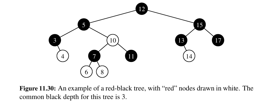
Formally, a red-black tree is a binary search tree (see Section 11.1) with nodes colored red and black in a way that satisfies the following properties:
Root Property: The root is black.
Red Property: The children of a red node (if any) are black.
Depth Property: All nodes with zero or one children have the same black depth, defined as the number of black ancestors. (Recall that a node is its own ancestor).
Red-Black Tree Operations
TODO: Not urgent
...
Insertion
TODO: Not urgent
...
Deletion
TODO: Not urgent
...
Performance of Red-Black Trees
• Proposition 11.10: The insertion of an item in a red-black tree storing \(n\) items can be done in \(O(log n)\) time and requires \(O(log n)\) recolorings and at most one trinode restructuring.
• Proposition 11.11: The algorithm for deleting an item from a red-black tree with \(n\) items takes \(O(log n)\) time and performs \(O(log n)\) recolorings and at most two restructuring operations.
Python Implementation
TODO: Not urgent
...
Here is the code to check out:
Incredible job.
Let's discover Sorting and Selection 🎱