Recursion 🍒
Recursion is a technique by which a function makes one or more calls to itself during execution.
File System, A Ruler, Binary Search and Fibonacci are great examples.
Illustrative Examples
Let's start by working on a factorial.
The factorial function is important because it is known to equal the number of ways in which n distinct items can be arranged into a sequence, that is, the number of permutations of n items.
For example, the three characters a, b, and c can be arranged in \(3! = 3 · 2 · 1 = 6\) ways: abc, acb, bac, bca, cab, and cba.
def factorial(n):
    # base case
    if n == 0:
        return 1
    # recursive case
    else:
        return n * factorial(n - 1)
Recursion is always with a base case and recursive case.
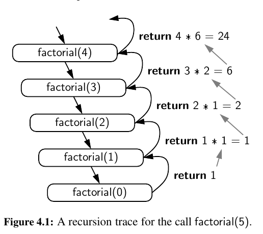
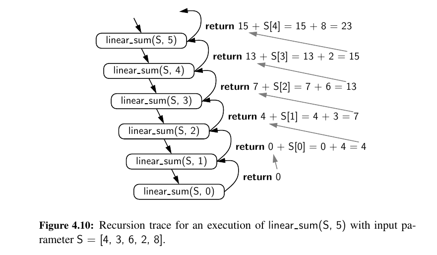
We illustrate the execution of a recursive function using a recursion trace.
Each entry of the trace corresponds to a recursive call. Each new recursive function call is indicated by a downward arrow to a new invocation.
When the function returns, an arrow showing this return is drawn and the return value may be indicated alongside this arrow.
In Python, each time a function (recursive or otherwise) is called, a structure known as an activation record or frame is made to store information about the progress of that invocation of the function.
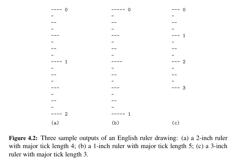
Let's move on to an English Ruler. 📏
There will be major and minor ticks on the ruler so that we can measure length.
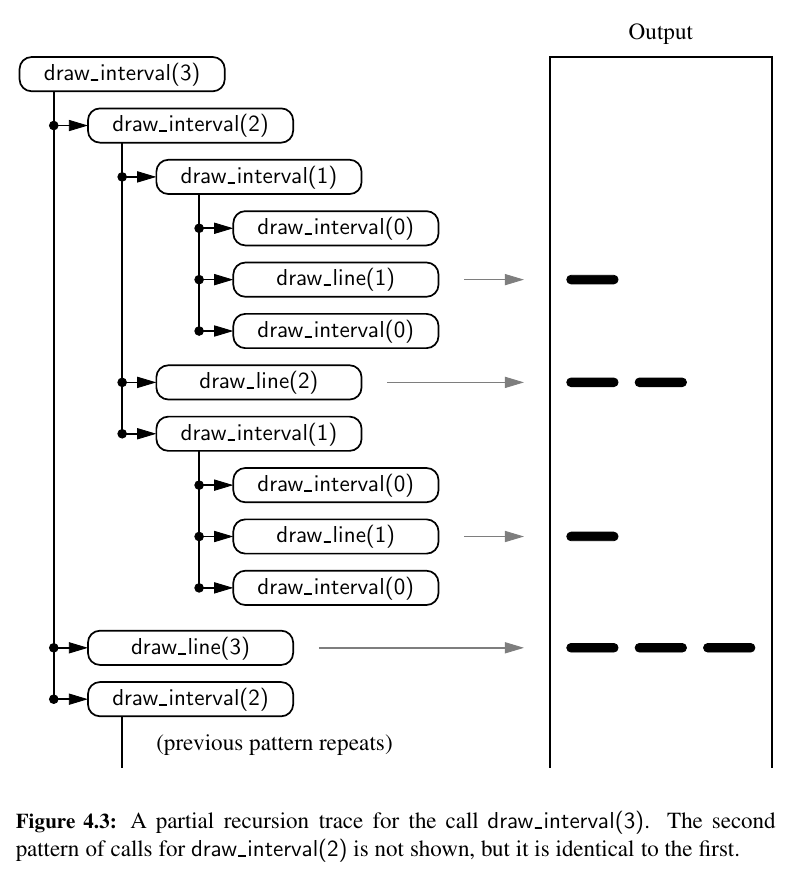
In general, an interval with a central tick length \(L ≥ 1\) is composed of:
- An interval with a central tick length \(L − 1\)
- A single tick of length \(L\)
- An interval with a central tick length \(L − 1\)
Here is the code:
Result will be:
Here is the recursion trace for it:
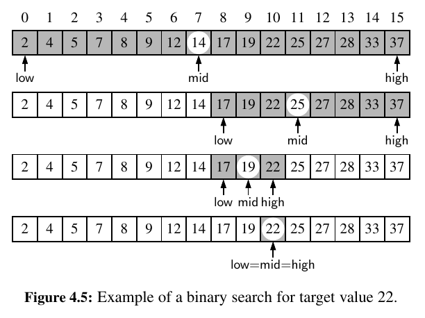
Next up, let's look at Binary Search:
It is among the most important of computer algorithms, and it is the reason that we so often store data in sorted order.
The algorithm maintains two parameters, low and high, such that all the candidate entries have index at least low and at most high.
Initially, low = 0 and high = n − 1. We then compare the target value to the median candidate, that is, the item data[mid] with index \(mid = floor((low + high)/2)\).
We consider three cases:
- If the target equals
data[mid], then we have found the item we are looking for, and the search terminates successfully. - If
target < data[mid], then we recur on the first half of the sequence, that is, on the interval of indices fromlowtomid − 1. - If
target > data[mid], then we recur on the second half of the sequence, that is, on the interval of indices frommid + 1tohigh.
An unsuccessful search occurs if low > high, as the interval [low, high] is empty.
Here is a recursive approach to binary search:
A picture is worth thousand of words:
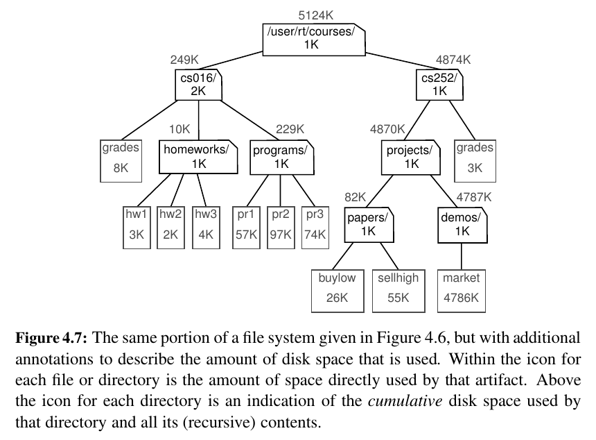
Let's look at File Systems 🥰:
Modern operating systems define file-system directories (which are also sometimes called “folders”) in a recursive way.
The disk space can be calculated recursively.
We will use Standard Library for our implementation in Python.
-
os.path.getsize(path): Return the immediate disk usage (measured in bytes) for the file or directory that is identified by the string path (e.g.,/user/rt/courses). -
os.path.isdir(path): Return True if entry designated by string path is a directory; False otherwise. -
os.listdir(path): Return a list of strings that are the names of all entries within a directory designated by string path. In our sample file system, if the parameter is/user/rt/courses, this returns the list["cs016" , "cs252"]. -
os.path.join(path, filename): Compose the path string and filename string using an appropriate operating system separator between the two (e.g., the / character for a Unix/Linux system, and the\character for Windows). Return the string that represents the full path to the file.
import os

def disk_usage(path):
    """Return the number of bytes used by a file/folder and any descendents"""
    total = os.path.getsize(path)
    if os.path.isdir(path):
        for filename in os.listdir(path):
            childpath = os.path.join(path, filename)
            total += disk_usage(childpath)
    print("{0:<7}".format(total), path)
    return total
The output can be something like:
disk_usage(os.path.join("/", "home", "sezai", "repository", "perfectHour"))
"""
5183    /home/sezai/repository/perfectHour/neetcode/007.is_valid_sudoku.py
2688    /home/sezai/repository/perfectHour/neetcode/042.find_the_duplicate_number.py
3370    /home/sezai/repository/perfectHour/neetcode/018.generate_parantheses.py
5018    /home/sezai/repository/perfectHour/neetcode/064.subsets.py
2254    /home/sezai/repository/perfectHour/neetcode/150.detect_squares.py
"""
Analyzing Recursive Algorithms - Invocation and Operations 🤔
We learned to analyze the efficiency of functions with big-Oh notation.
For recursive algorithms, we will look at the number of operations for each activation.
• Invocation: How many calls are made?
• Operation: How much execution is done?
The factorial function was:
This function has \(n+1\) activation's and constant operations for each of the activation. So overall time complexity is O(n).
In the binary search we perform constant number of primitive operations at each recursive call. So the time complexity is \(log(n)\).
Recursion Run Amok 😯
Run amok means, is to behave uncontrollably and disruptively.
Although recursion is a very powerful tool, it can easily be misused in various ways.
Let's revisit the element uniqueness problem:
def unique3(S, start, stop):
    """Return True if there are no duplicate elements in slice S[start:stop]."""
    if stop − start <= 1: return True  # at most one item
    elif not unique(S, start, stop−1): return False # first part has duplicate
    elif not unique(S, start+1, stop): return False # second part has duplicate
    else: return S[start] != S[stop−1] # do first and last differ?
Unfortunately, this is a terribly inefficient use of recursion.
The non recursive part of each call uses \(O(1)\) time, so the overall running time will be proportional to the total number of recursive invocations.
A single call to unique3 for a problem of size n may result in two recursive calls on problems of size \(n − 1.\)
Those two calls with size \(n − 1\) could in turn result in four calls (two each) with a range of size \(n − 2\), and thus eight calls with size \(n − 3\) and so on.
Thus, in the worst case, the total number of function calls is given by the geometric summation \(1 + 2 + 4 + · · · + 2^{n−1}\) which is equal to \(2^{n − 1}\) .
Thus, the running time of function unique3 is O(\(2^n\)).
This is an incredibly inefficient function for solving the element uniqueness problem.
Here is another example:
def bad_fibonacci(n):
    """Return the nth Fibonacci number."""
    if n <= 1:
        return n
    else:
        return bad_fibonacci(n−2) + bad_fibonacci(n−1)
Unfortunately, such a direct implementation of the Fibonacci formula results in a terribly inefficient function.
Computing the \(n_{th}\) Fibonacci number in this way requires an exponential number of calls to the function.
What can we do? 🤔
We can compute \(F_{n}\) much more efficiently using a recursion in which each invocation makes only one recursive call. To do so, we need to redefine the expectations of the function.
Rather than having the function return a single value, which is the nth Fibonacci number, we define a recursive function that returns a pair of consecutive Fibonacci numbers (\(F_n, F_{n−1}\)), using the convention \(F_{−1} = 0\).
def good_fibonacci(n):
    """Return pair of Fibonacci numbers, F(n) and F(n-1)."""
    if n <= 1:
        return (n,0)
    else:
        (a, b) = good_fibonacci(n−1)
        return (a+b, a)

good_fibonacci(10) # (55, 34)
Or using a map to store all values and return a single one:
def fib(n, memo = {}):
    if n <= 1:
        return n
    # check if the result is already calculated
    if n not in memo:
        # If not, calculate and store the result
        memo[n] = fib(n-1, memo) + fib(n-2, memo)
    return memo[n]

fib(10) # 55
fib(17) # 1597
or we can use lru_cache:
from functools import lru_cache

@lru_cache
def fibo_cached(n):
    if n <= 1:
        return n
    else:
        n = fibo_cached(n-1) + fibo_cached(n-2)
        return n

fibo_cached(10) # 55
Maximum Recursive Depth in Python 🔎
Another danger in the misuse of recursion is known as infinite recursion. 😮
If each recursive call makes another recursive call, without ever reaching a base case, then we have an infinite series of such calls.
This is a fatal error.
Tip
A programmer should ensure that each recursive call is in some way progressing toward a base case (for example, by having a parameter value that decreases with each call).
However, to combat against infinite recursions, the designers of Python made an intentional decision to limit the overall number of function activations that can be simultaneously active.
The precise value of this limit depends upon the Python distribution, but a typical default value is 1000.
import sys
old = sys.getrecursionlimit() # perhaps 1000 is typical
sys.setrecursionlimit(1000000) # change to allow 1 million nested calls
Further into Recursion 👨💻
We organize our presentation by considering the maximum number of recursive calls that may be started from within the body of a single activation.
• If a recursive call starts at most one other, we call this a linear recursion. • If a recursive call may start two others, we call this a binary recursion. • If a recursive call may start three or more others, this is multiple recursion.
Linear Recursion
If a recursive function is designed so that each invocation of the body makes at most one new recursive call, this is know as linear recursion.
Of the recursions we have seen so far, the implementation of the factorial function and the good_fibonacci function are clear examples of linear recursion.
The linear recursion terminology reflects the structure of the recursion trace, not the running time.
def linear_sum(S, n):
    """Return the sum of the first n numbers of sequence S."""
    if n == 0:
        return 0
    else:
        return linear sum(S, n−1) + S[n−1]
Constant operation for \(n + 1\) activations. So the overall time complexity is \(O(n)\).
Here is a \(O(n)\) time power function using recursion:
def power(x,n):
    """Compute the value of x**n for integer n"""
    if n == 0:
        return 1
    else:
        return x * power(x, n - 1)
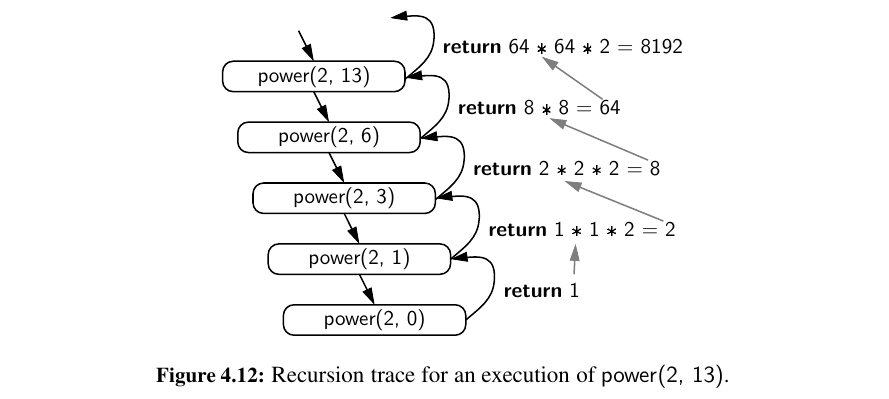
Here is a even better version, running at \(O(log(n))\):
def power(x, n):
    """Compute the value x n for integer n."""
    if n == 0:
        return 1
    else:
        partial = power(x, n // 2) # rely on truncated division
        result = partial * partial
        if n % 2 == 1:   # if n odd, include extra factor of x
            result *= x
        return result
Binary Recursion
When a function makes two recursive calls, we say that it uses binary recursion.
We have already seen several examples of binary recursion, most notably when drawing the English ruler or in the bad_fibonacci function.
Here is another interesting example, binary sum:
Although binary sum has \(2^n\) recursive calls, the time complexity is \(O(n)\) because at each call \(n\) is halved. You can think it as: \(2^{(log2^n)} = n\)
Multiple Recursion
Generalizing from binary recursion, we define multiple recursion as a process in which a function may make more than two recursive calls.
Our recursion for analyzing the disk space usage of a file system is an example of multiple recursion, because the number of recursive calls made during one invocation was equal to the number of entries within a given directory of the file system.
Another common application of multiple recursion is when we want to enumerate various configurations in order to solve a combinatorial puzzle.
For example, the following are all instances of what are known as summation puzzles:
# Algorithm PuzzleSolve(k,S,U):
#   Input: An integer k, sequence S, and set U
#   Output: An enumeration of all k-length extensions to S using elements in U
#       without repetitions
#   for each e in U do
#       Add e to the end of S
#       Remove e from U {e is now being used}
#       if k = =  1 then
#           Test whether S is a configuration that solves the puzzle
#           if S solves the puzzle then
#           return “Solution found: ” S
#       else
#           PuzzleSolve(k−1,S,U) {a recursive call}
#       Remove e from the end of S
#       Add e back to U {e is now considered as unused}
Designing Recursive Algorithms
In general, an algorithm that uses recursion typically has the following form:
• Test for base cases. We begin by testing for a set of base cases (there should be at least one). These base cases should be defined so that every possible chain of recursive calls will eventually reach a base case, and the handling of each base case should not use recursion.
• Recur. If not a base case, we perform one or more recursive calls. This recursive step may involve a test that decides which of several possible recursive calls to make. We should define each possible recursive call so that it makes progress towards a base case.
To design a recursive algorithm for a given problem, it is useful to think of the different ways we might define subproblems that have the same general structure as the original problem.
If one has difficulty finding the repetitive structure needed to design a recursive algorithm, it is sometimes useful to work out the problem on a few concrete examples to see how the subproblems should be defined.
Eliminating Tail Recursion 💕
The main benefit of a recursive approach to algorithm design is that it allows us to succinctly take advantage of a repetitive structure present in many problems.
However, the usefulness of recursion comes at a modest cost.
In particular, the Python interpreter must maintain activation records that keep track of the state of each nested call.
When computer memory is at a premium, it is useful in some cases to be able to derive non recursive algorithms from recursive ones.
Some forms of recursion can be eliminated without any use of axillary memory. A notable such form is known as tail recursion.
A recursion is a tail recursion if any recursive call that is made from one context is the very last operation in that context, with the return value of the recursive call (if any) immediately returned by the enclosing recursion.
Any tail recursion can be re implemented non recursively by enclosing the body in a loop for repetition, and replacing a recursive call with new parameters by a reassignment of the existing parameters to those values.
Here is an example of reversing a sequence recursively.
def reverse(S, start, stop):
    """Reverse elements in implicit slice S[start:stop]."""
    if start < stop - 1: # if at least 2 elements:
        S[start], S[stop-1] = S[stop-1], S[start] # swap first and last
        reverse(S, start+1, stop-1) # recur on rest
Here is the iterative version (using two pointers 😮):
def reverse_iterative(S):
    """Reverse elements in sequence S."""
    start, stop = 0, len(S)
    while start < stop -1:
        S[start], S[stop-1] = S[stop-1], S[start] # swap first and last
        start, stop = start + 1, stop -1 # narrow the range
So it's possible to find loop-based equivalents for tail-recursive algorithms — reducing the risk of stack overflow and often improving performance.
This is especially valuable in systems programming, real-time systems, or any environment where memory is constrained.
You are doing great! Let's move on to Array Based Sequences 🥳