Maps, Hash Tables and Skip Lists¶

Maps and Dictionaries 😍¶

Python’s dict class is arguably the most significant data structure in the language.

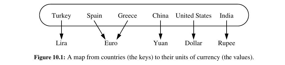
It represents an abstraction known as a dictionary in which unique keys are mapped to associated values.

Because of the relationship they express between keys and values, dictionaries are commonly known as associative arrays or maps.

Common applications of maps include the following:

• A university’s information system relies on some form of a student ID as a key that is mapped to that student’s associated record (such as the student’s name, address, and course grades) serving as the value.

• The domain-name system (DNS) maps a host name, such as www.wiley.com, to an Internet-Protocol (IP) address, such as 208.215.179.146 (DNS locates and serves the web page you’re looking for in a matter of seconds through a rapid, complex series of internet protocols. It's like a phone book for the web.).

• A social media site typically relies on a (non numeric) username as a key that can be efficiently mapped to a particular user’s associated information.

• A computer graphics system may map a color name, such as turquoise , to the triple of numbers that describes the color’s RGB (red-green-blue) representation, such as (64,224,208).

• Python uses a dictionary to represent each namespace, mapping an identifying string, such as pi , to an associated object, such as 3.14159.

The Map ADT¶

Here is the map ADT and it's methods:

Method	Explained
`M[k]`	Return the value v associated with key k in map M, if one exists; otherwise raise a `KeyError`. In Python, this is implemented with the special method `__getitem__` .
`M[k] = v`	Associate value v with key k in map M, replacing the existing value if the map already contains an item with key equal to k. In Python, this is implemented with the special method `__setitem__`.
`del M[k]`	Remove from map M the item with key equal to k; if M has no such item, then raise a `KeyError`. In Python, this is implemented with the special method `__delitem__` .
`len(M)`	Return the number of items in map M. In Python, this is implemented with the special method `__len__` .
`iter(M)`	The default iteration for a map generates a sequence of keys in the map. In Python, this is implemented with the special method `__iter__` , and it allows loops of the form, for k in M.
`k in M`:	Return `True` if the map contains an item with key k. In Python, this is implemented with the special contains method.
`M.get(k, d=None)`	Return `M[k]` if key k exists in the map; otherwise return default value d. This provides a form to query `M[k]` without risk of a `KeyError`.
`M.setdefault(k, d)`	If key k exists in the map, simply return `M[k]`; if key k does not exist, set `M[k] = d` and return that value.
`M.pop(k, d=None)`	Remove the item associated with key k from the map and return its associated value v. If key k is not in the map, return default value d (or raise `KeyError` if parameter d is `None`).
`M.popitem()`	Remove an arbitrary key-value pair from the map, and return a (k,v) tuple representing the removed pair. If map is empty, raise a `KeyError`.
`M.clear()`	Remove all key-value pairs from the map.
`M.keys()`	Return a set-like view of all keys of M.
`M.values()`	Return a set-like view of all values of M.
`M.items():`	Return a set-like view of (k,v) tuples for all entries of M.
`M.update(M2)`	Assign `M[k] = v` for every (k,v) pair in map M2.
`M == M2`	Return True if maps M and M2 have identical key-value associations.
`M != M2`	Return True if maps M and M2 do not have identical key-value associations.

operations_on_a_map — Series of Operations for a Map

Application: Counting Word Frequencies¶

As a case study for using a map, consider the problem of counting the number of occurrences of words in a document.

This is a standard task when performing a statistical analysis of a document, for example, when categorizing an email or news article.

freq = {}
for piece in open(filename).read().lower().split():
    # only consider alphabetic characters within this piece
    word = "".join(c for c in piece if c.isalpha())
    if word: # require at least one alphabetic character
        freq[word] = 1 + freq.get(word, 0)

max_word = ""
max_count = 0
# tuple traversing
for (w,c) in freq.items(): # (key, value) tuples represent (word, count)
    if c > max count:
        max_word = w
        max_count = c
print( "The most frequent word is ", max word)
print( "Its number of occurrences is ", max count)

Application: Finding The min/max Value based on values of dict¶

Although Python dict's iterate over their keys, we can define max()/min() with the help of key parameter, such that we are able make comparisons based on values:

d = {100:2, 4:45, 7:78, 3: 123}

max(d, key= lambda x: d[x]) # 3

min(d) # 3

min(d, key = lambda x : d[x]) # 100

Python’s `MutableMapping` Abstract Base Class¶

The collections module provides two abstract base classes that are relevant to our current discussion: the Mapping and MutableMapping classes.

What we define as the map ADT in Chapter 10.1.1 is akin to the MutableMapping abstract base class in Python’s collections module.

The significance of these abstract base classes is that they provide a framework to assist in creating a user-defined map class.

In particular, the MutableMapping class provides concrete implementations for all behaviors other than the first five outlined in Chapter 10.1.1: __getitem__ , __setitem__ , __delitem__ , len , and __iter__ .

As we implement the map abstraction with various data structures, as long as we provide the five core behaviors, we can inherit all other derived behaviors by simply declaring MutableMapping as a parent class.

Our `MapBase` Class¶

We will be providing many different implementations of the map ADT, in the remainder of this chapter and next, using a variety of data structures demonstrating a trade-off of advantages and disadvantages.

hierarchy_of_maps — Our Hierarchy for Maps

Here is the MapBase:

map_base.py
from collections import MutableMapping

class MapBase(MutableMapping):
  """Our own abstract base class that includes a nonpublic _Item class."""

  #------------------------ nested _Item class --------------------------#
  class _Item:
    __slots__ = '_key', '_value'

    def __init__(self, k, v):
      self._key = k
      self._value = v

    def __equal__(self, other):
      """Compare items based on their keys."""
      return self._key == other._key

    def __ne__(self, other):
      """Not equal."""
      return not (self == other)

    def __lt__(self, other):
      """Less than Comparison for keys."""
      return self._key < other._key

    def __repr__(self):
      return "key %s value %s" % (self._key, self._value)

Simple Unsorted Map Implementation¶

An empty table is initialized as self._table within the constructor for our map. Can we use a python list ?

This list-based map implementation is simple, but it is not particularly efficient.

Each of the fundamental methods, __getitem__ , __setitem__ , and __delitem__ , relies on a for loop to scan the underlying list of items in search of a matching key.

list_based_map.py
class UnsortedTableMap(MapBase):
    """Map implementation using an unordered list."""

    def __init__(self):
        """Create an empty map."""
        self._table = []  # list of _Item's

    def __getitem__(self, k):
        """Return value associated with key k (raise KeyError if not found)."""
        for item in self._table:
            if k == item._key:
                return item._value
        raise KeyError('Key Error: ' + repr(k))

    def __setitem__(self, k, v):
        """Assign value v to key k, overwriting existing value if present."""
        for item in self._table:
            if k == item._key:  # Found a match:
                item._value = v  # reassign value
                return  # and quit
        # did not find match for key
        self._table.append(self._Item(k, v))

    def __delitem__(self, k):
        """Remove item associated with key k (raise KeyError if not found)."""
        for j in range(len(self._table)):
            if k == self._table[j]._key:  # Found a match:
                self._table.pop(j)  # remove item
                return  # and quit
        raise KeyError('Key Error: ' + repr(k))

    def __len__(self):
        """Return number of items in the map."""
        return len(self._table)

    def __iter__(self):
        """Generate iteration of the map's keys."""
        for item in self._table:
            yield item._key  # yield the KEY

Hash Tables¶

In this section, we introduce one of the most practical data structures for implementing a map, and the one that is used by Python’s own implementation of the dict class.

This structure is known as a hash table.

Intuitively, a map M supports the abstraction of using keys as indices with a syntax such as M[k].

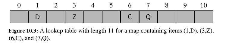
There are two challenges in extending this framework to the more general setting of a map.

First, we may not wish to devote an array of length N if it is the case that $N >> n$.

Second, we do not in general require that a map’s keys be integers.

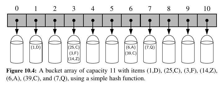
The novel concept for a hash table is the use of a hash function to map general keys to corresponding indices in a table.

Ideally, keys will be well distributed in the range from $0$ to $N − 1$ by a hash function, but in practice there may be two or more distinct keys that get mapped to the same index.

We will conceptualize our table as a bucket array, as shown in Figure 10.4, in which each bucket may manage a collection of items that are sent to a specific index by the hash function.

Hash Functions¶

The goal of a hash function, $h$, is to map each key $k$ to an integer in the range [0, N − 1], where $N$ is the capacity of the bucket array for a hash table.

If there are two or more keys with the same hash value, then two different items will be mapped to the same bucket in A.

In this case, we say that a collision has occurred. To be sure, there are ways of dealing with collisions, which we will discuss later, but the best strategy is to try to avoid them in the first place.

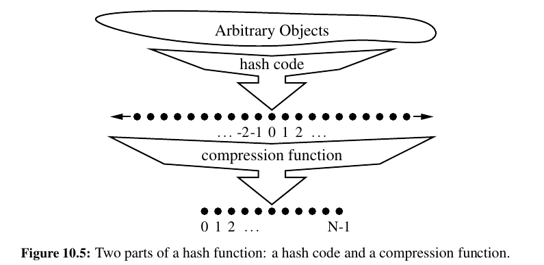
It is common to view the evaluation of a hash function, $h(k)$, as consisting of two portions—a hash code that maps a key k to an integer.

And a compression function that maps the hash code to an integer within a range of indices, $[0, N − 1]$, for a bucket array.

Hash Codes¶

The first action that a hash function performs is to take an arbitrary key k in our map and compute an integer that is called the hash code for k; this integer need not be in the range $[0, N − 1]$, and may even be negative.

We desire that the set of hash codes assigned to our keys should avoid collisions as much as possible.

For if the hash codes of our keys cause collisions, then there is no hope for our compression function to avoid them.

Treating the Bit Representation as an Integer¶

To begin, we note that, for any data type X that is represented using at most as many bits as our integer hash codes, we can simply take as a hash code for X an integer interpretation of its bits.

For example, the hash code for key 314 could simply be 314.

Not a good idea.

Python relies on 32-bit hash codes. If a floating-point number uses a 64-bit representation, its bits cannot be viewed directly as a hash code.

One possibility is to use only the high-order 32 bits (or the low-order 32 bits).

This hash code, of course, ignores half of the information present in the original key, and if many of the keys in our map only differ in these bits, then they will collide using this simple hash code.

Polynomial Hash Codes¶

The summation and exclusive-or hash codes, described above, are not good choices for character strings or other variable-length objects that can be viewed as tuples of the form $(x_0, x_1 , . . . , x_{n−1})$, where the order of the $x_i$ ’s is significant.

For example, consider a 16-bit hash code for a character string s that sums the Unicode values of the characters in s.

This hash code unfortunately produces lots of unwanted collisions for common groups of strings. In particular, "temp01" and "temp10" collide using this function, as do "stop", "tops", "pots", and "spot".

A better hash code should somehow take into consideration the positions of the $x_i$ ’s.

\[ x_0 a^{n−1} + x_1 a^{n−2} + · · · + x_{n−2} a + x_{n−1} . \]

Mathematically speaking, this is simply a polynomial in a that takes the components $(x_0, x_1 , . . . , x_{n−1} )$ of an object $x$ as its coefficients. This hash code is therefore called a polynomial hash code.

Intuitively, a polynomial hash code uses multiplication by different powers as a way to spread out the influence of each component across the resulting hash code.

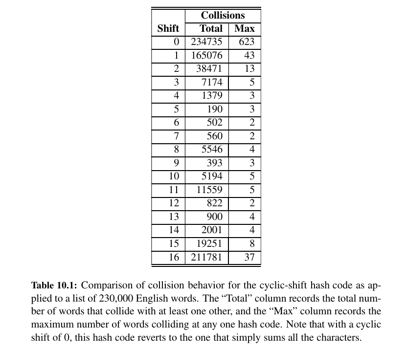
Cyclic-Shift Hash Codes¶

A variant of the polynomial hash code replaces multiplication by a with a cyclic shift of a partial sum by a certain number of bits.

For example, a 5-bit cyclic shift of the 32-bit value 00111101100101101010100010101000 is achieved by taking the leftmost five bits and placing those on the rightmost side of the representation, resulting in 10110010110101010001010100000111.

While this operation has little natural meaning in terms of arithmetic, it accomplishes the goal of varying the bits of the calculation.

def hash_code(s):
    mask = (1<<32) -1
    h = 0
    for character in s:
        h = (h << 5 & mask) | (h >> 27)
        h += ord(character)
    return h

print(hash_code("a")) # 97
print(hash_code("5")) # 53
print(hash_code("88")) # 1848

As with the traditional polynomial hash code, fine-tuning is required when using a cyclic-shift hash code, as we must wisely choose the amount to shift by for each new character.

collisions_on_cyclic_shift — Collisions for Cyclic Shift Hash Codes

Hash Codes in Python 🥳¶

The standard mechanism for computing hash codes in Python is a built-in function with signature hash(x) that returns an integer value that serves as the hash code for object x.

However, only immutable (int, float, str, bool, tuple, etc.) data types are deemed hashable in Python.

This restriction is meant to ensure that a particular object’s hash code remains constant during that object’s lifespan.

This is an important property for an object’s use as a key in a hash table.

A problem could occur if a key were inserted into the hash table, yet a later search were performed for that key based on a different hash code than that which it had when inserted; the wrong bucket would be searched.

Instances of user-defined classes are treated as unhashable by default, with a TypeError raised by the hash function.

However, a function that computes hash codes can be implemented in the form of a special method named __hash__ within a class.

The returned hash code should reflect the immutable attributes of an instance. It is common to return a hash code that is itself based on the computed hash of the combination of such attributes.

For example, a Color class that maintains three numeric red, green, and blue components might implement the method as:

def __hash__(self):
    return hash((self._red, self._green, self._blue)) # # hash combined tuple

An important rule to obey is that if a class defines equivalence through __eq__ , then any implementation of __hash__ must be consistent, in that if x == y, then hash(x) == hash(y).

This rule extends to any well-defined comparisons between objects of different classes.

For example, since Python treats the expression 5 == 5.0 as true, it ensures that hash(5) and hash(5.0) are the same.

Compression Functions 😍¶

We talked about hash codes so far. But we still have to map the value we found to the array.

The hash code for a key k will typically not be suitable for immediate use with a bucket array, because the integer hash code may be negative or may exceed the capacity of the bucket array.

The Division Method¶

A simple compression function is the division method, which maps an integer i to $i \:mod \:N$ where N, the size of the bucket array, is a fixed positive integer.

The MAD Method¶

A more sophisticated compression function, which helps eliminate repeated patterns in a set of integer keys, is the Multiply-Add-and-Divide (or “MAD”) method.

This method maps an integer $i$ to $$ [(ai + b)\:mod p]\:mod N, $$

where N is the size of the bucket array, p is a prime number larger than $N$, and $a$ and $b$ are integers chosen at random from the interval $[0, p − 1]$, with $a$ > 0.

Collision-Handling Schemes 🍒¶

The main idea of a hash table is to take a bucket array, A, and a hash function, h, and use them to implement a map by storing each item (k, v) in the “bucket” $A[h(k)]$.

This simple idea is challenged, however, when we have two distinct keys, $k1$ and $k2$ , such that h(k1) = h(k2).

The existence of such collisions prevents us from simply inserting a new item (k, v) directly into the bucket $A[h(k)]$.

It also complicates our procedure for performing insertion, search, and deletion operations.

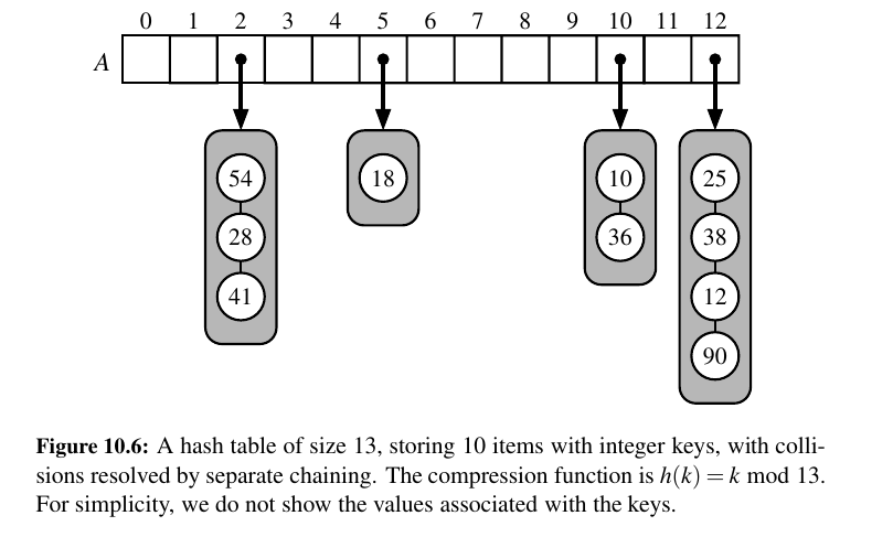
Separate Chaining¶

A simple and efficient way for dealing with collisions is to have each bucket A[j] store its own secondary container, holding items (k, v) such that $h(k) = j$.

A natural choice for the secondary container is a small map instance implemented using a list.

In the worst case, operations on an individual bucket take time proportional to the size of the bucket.

Assuming we use a good hash function to index the n items of our map in a bucket array of capacity $N$, the expected size of a bucket is $n/N$.

Therefore, if given a good hash function, the core map operations run in $O(⌈n/N⌉)$.

The ratio $λ = n/N$, called the ==load factor== of the hash table, should be bounded by a small constant, preferably below 1.

As long as λ is $O(1)$, the core operations on the hash table run in $O(1)$ expected time.

If we go over a certain Load Factor, we resize bucket array. Python's threshold for load factor is 2/3.

Open Addressing¶

The separate chaining rule has many nice properties, such as affording simple implementations of map operations, but it nevertheless has one slight disadvantage: It requires the use of an auxiliary data structure—a list—to hold items with colliding keys.

If space is at a premium (for example, if we are writing a program for a small handheld device), then we can use the alternative approach of always storing each item directly in a table slot.

This approach saves space because no auxiliary structures are employed, but it requires a bit more complexity to deal with collisions. There are several variants of this approach, collectively referred to as open addressing schemes, which we discuss next.

Open addressing requires that the load factor is always at most 1 and that items are stored directly in the cells of the bucket array itself.

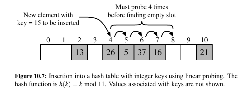
Linear Probing and Its Variants - Open Addressing Methods 💕¶

With this approach, if we try to insert an item $(k, v)$ into a bucket A[j] that is already occupied, where $j = h(k)$, then we next try $A[( j + 1) \: mod N].$ If $A[( j + 1) \: mod N]$ is also occupied, then we try $A[( j + 2) \: mod N]$, and so on, until we find an empty bucket that can accept the new item.

Tip

Linear Probing -> Keep probing until you find a spot.

Problem with linear probing is that, you cannot just delete an item.

Instead, make them available:

To implement a deletion, we cannot simply remove a found item from its slot in the array.

For example, after the insertion of key 15 portrayed in Figure 10.7, if the item with key 37 were trivially deleted, a subsequent search for 15 would fail because that search would start by probing at index 4, then index 5, and then index 6, at which an empty cell is found.

A typical way to get around this difficulty is to replace a deleted item with a special “available” marker object.

With this special marker possibly occupying spaces in our hash table, we modify our search algorithm so that the search for a key k will skip over cells containing the available marker and continue probing until reaching the desired item or an empty bucket (or returning back to where we started from).

Linear probing saves memory space but slows us down. 😕

Although use of an open addressing scheme can save space, linear probing suffers from an additional disadvantage.

It tends to cluster the items of a map into contiguous runs, which may even overlap (particularly if more than half of the cells in the hash table are occupied). Such contiguous runs of occupied hash cells cause searches to slow down considerably.

Quadratic Probing¶

Another open addressing strategy, known as quadratic probing, iteratively tries the buckets $A[(h(k) + f (i)) \: mod N]$, for $i = 0, 1, 2, . . .,$ where $f (i) = i^2$, until finding an empty bucket.

As with linear probing, the quadratic probing strategy complicates the removal operation, but it does avoid the kinds of clustering patterns that occur with linear probing.

Double Hashing 💖¶

Tip

This is what Python dict use (kinda)!

Python dictionaries use a form of open addressing with a technique similar to double hashing for collision resolution — but it’s not classical double hashing as seen in textbooks.

The algorithm used in CPython is sometimes described as "perturbed probing", and it is more sophisticated than naive double hashing. In CPython, the logic for dictionary probing is located in CPython GitHub Repo — dictobject.c,

An open addressing strategy that does not cause clustering of the kind produced by linear probing or the kind produced by quadratic probing is the double hashing strategy.

In this approach, we choose a secondary hash function, $h'$, and if $h$ maps some key $k$ to a bucket $A[h(k)]$ that is already occupied, then we iteratively try the buckets $A[(h(k) + f (i)) \: mod N]$ next, for $i = 1, 2, 3, . . .,$ where $f (i) = i · h' (k)$.

In this scheme, the secondary hash function is not allowed to evaluate to zero; a common choice is $h' (k) = q − (k \: mod q)$, for some prime number $q < N$. Also, $N$ should be a prime.

Another approach to avoid clustering with open addressing is to iteratively try buckets $A[(h(k) + f (i)) \: mod N]$ where $f(i)$ is based on a pseudo-random number generator, providing a repeatable, but somewhat arbitrary, sequence of subsequent probes that depends upon bits of the original hash code.

This is the approach currently used by Python’s dictionary class.

Load Factors, Rehashing, and Efficiency 😯¶

In the hash table schemes described so far, it's important that the load factor, $λ = n/N$, be kept below 1.

With separate chaining, as λ gets very close to 1, the probability of a collision greatly increases, which adds overhead to our operations, since we must revert to linear-time list-based methods in buckets that have collisions.

Experiments and average-case analyses suggest that we should maintain λ < 0.9 for hash tables with separate chaining.

With open addressing, on the other hand, as the load factor λ grows beyond 0.5 and starts approaching 1, clusters of entries in the bucket array start to grow as well.

These clusters cause the probing strategies to “bounce around” the bucket array for a considerable amount of time before they find an empty slot.

We explore the degradation of quadratic probing when λ ≥ 0.5.

Experiments suggest that we should maintain λ < 0.5 for an open addressing scheme with linear probing, and perhaps only a bit higher for other open addressing schemes (for example, Python’s implementation of open addressing enforces that λ < 2/3).

If load factor goes over threshold, resize the table:

If an insertion causes the load factor of a hash table to go above the specified threshold, then it is common to resize the table (to regain the specified load factor) and to reinsert all objects into this new table.

Although we need not define a new hash code for each object, we do need to reapply a new compression function that takes into consideration the size of the new table

Efficiency of Hash Tables 🤔¶

In the worst case, a poor hash function could map every item to the same bucket.

This would result in linear-time performance for the core map operations with separate chaining, or with any open addressing model in which the secondary sequence of probes depends only on the hash code.

Operation	List	Hash Table Expected	Hash Table Worst
`__getitem__`	$O(n)$	$O(1)$	$O(n)$
`__setitem__`	$O(n)$	$O(1)$	$O(n)$
`__delitem__`	$O(n)$	$O(1)$	$O(n)$
`__len__`	$O(1)$	$O(1)$	$O(1)$
`__iter__`	$O(n)$	$O(n)$	$O(n)$

Table: Comparison of the running times of the methods of a map realized by means of an unsorted list (as in Chapter 10.1.5) or a hash table.

We let n denote the number of items in the map, and we assume that the bucket array supporting the hash table is maintained such that its capacity is proportional to the number of items in the map.

Tip

Here is some wisdom about hash tables.

In practice, hash tables are among the most efficient means for implementing a map, and it is essentially taken for granted by programmers that their core operations run in constant time.

Python’s dict class is implemented with hashing, and the Python interpreter relies on dictionaries to retrieve an object that is referenced by an identifier in a given namespace. (See Chapter 1.10 and 2.5.)

The basic command c = a + b`` involves two calls togetitemin the dictionary for the local namespace to retrieve the values identified as a and b, and a call tosetitem` to store the result associated with name c in that namespace.

In our own algorithm analysis, we simply presume that such dictionary operations run in constant time, independent of the number of entries in the namespace (Admittedly, the number of entries in a typical namespace can almost surely be bounded by a constant.).

Python Hash Table Implementation¶

We extend the MapBase class (from Code Fragment 10.2), to define a new HashMapBase class providing much of the common functionality to our two hash table implementations.

• The bucket array is represented as a Python list, named self._table, with all entries initialized to None.

• We maintain an instance variable self._n that represents the number of distinct items that are currently stored in the hash table.

• If the load factor of the table increases beyond 0.5, we double the size of the table and rehash all items into the new table.

• We define a hash function utility method that relies on Python’s built-in hash function to produce hash codes for keys, and a randomized Multiply-Add-and-Divide (MAD) formula for the compression function.

In our design, the HashMapBase class presumes the following to be abstract methods, which must be implemented by each concrete subclass:

• _bucket_getitem(j, k): This method should search bucket j for an item having key k, returning the associated value, if found, or else raising a KeyError.

• _bucket_setitem(j, k, v): This method should modify bucket j so that key k becomes associated with value v. If the key already exists, the new value overwrites the existing value. Otherwise, a new item is inserted and this method is responsible for incrementing self._n.

• _bucket_delitem(j, k) : This method should remove the item from bucket j having key k, or raise a KeyError if no such item exists. (self. n is decremented after this method.)

• __iter__ : This is the standard map method to iterate through all keys of the map. Our base class does not delegate this on a per-bucket basis because “buckets” in open addressing are not inherently disjoint.

hash_map_base.py
class HashMapBase(MapBase):
    """Abstract base class for map using hash-table with MAD compression.
    Keys must be hashable and non-None.
    """
    def __init__(self, cap=11, p=109345121):
        """Create an empty hash-table map.
        cap     initial table size (default 11)
        p       positive prime used for MAD (default 109345121)
        """
        self._table = cap * [None]
        self._n = 0  # number of entries in the map
        self._prime = p  # prime for MAD compression
        self._scale = 1 + randrange(p - 1)  # scale from 1 to p-1 for MAD
        self._shift = randrange(p)  # shift from 0 to p-1 for MAD

    def _hash_function(self, k):
        return (hash(k) * self._scale + self._shift) % self._prime % len(self._table)

    def __len__(self):
        return self._n

    def __getitem__(self, k):
        j = self._hash_function(k)
        return self._bucket_getitem(j, k)  # may raise KeyError

    def __setitem__(self, k, v):
        j = self._hash_function(k)
        self._bucket_setitem(j, k, v)  # subroutine maintains self._n
        if self._n > len(self._table) // 2:  # keep load factor <= 0.5
            self._resize(2 * len(self._table) - 1)  # number 2^x - 1 is often prime

    def __delitem__(self, k):
        j = self._hash_function(k)
        self._bucket_delitem(j, k)  # may raise KeyError
        self._n -= 1

    def _resize(self, c):
        """Resize bucket array to capacity c and rehash all items."""
        old = list(self.items())  # use iteration to record existing items
        self._table = c * [None]  # then reset table to desired capacity
        self._n = 0  # n recomputed during subsequent adds
        for (k, v) in old:
            self[k] = v  # reinsert old key-value pair

Separate Chaining Implementation¶

A concrete implementation of a hash table with separate chaining.

chain_hash_map.py
class ChainHashMap(HashMapBase):
    """Hash map implemented with separate chaining for collision resolution."""
    def _bucket_getitem(self, j, k):
        bucket = self._table[j]
        if bucket is None:
            raise KeyError('Key Error: ' + repr(k))  # no match found
        return bucket[k]  # may raise KeyError

    def _bucket_setitem(self, j, k, v):
        if self._table[j] is None:
            self._table[j] = UnsortedTableMap()  # bucket is new to the table
        oldsize = len(self._table[j])
        self._table[j][k] = v
        if len(self._table[j]) > oldsize:  # key was new to the table
            self._n += 1  # increase overall map size

    def _bucket_delitem(self, j, k):
        bucket = self._table[j]
        if bucket is None:
            raise KeyError('Key Error: ' + repr(k))  # no match found
        del bucket[k]  # may raise KeyError

    def __iter__(self):
        for bucket in self._table:
            if bucket is not None:  # a nonempty slot
                for key in bucket:
                    yield key

Linear Probing Implementation¶

Our implementation of a ProbeHashMap class, using open addressing with linear probing, is down below.

In order to support deletions, we use a technique described before, in which we place a special marker in a table location at which an item has been deleted, so that we can distinguish between it and a location that has always been empty.

probe_hash_map.py
class ProbeHashMap(HashMapBase):
    """Hash map implemented with linear probing for collision resolution."""
    _AVAIL = object()  # sentinal marks locations of previous deletions

    def _is_available(self, j):
        """Return True if index j is available in table."""
        return self._table[j] is None or self._table[j] is ProbeHashMap._AVAIL

    def _find_slot(self, j, k):
        """Search for key k in bucket at index j.

        Return (success, index) tuple, described as follows:
        If match was found, success is True and index denotes its location.
        If no match found, success is False and index denotes first available slot.
        """
        firstAvail = None
        while True:
            if self._is_available(j):
                if firstAvail is None:
                    firstAvail = j  # mark this as first avail
                if self._table[j] is None:
                    return (False, firstAvail)  # search has failed
            elif k == self._table[j]._key:
                return (True, j)  # found a match
            j = (j + 1) % len(self._table)  # keep looking (cyclically)

    def _bucket_getitem(self, j, k):
        found, s = self._find_slot(j, k)
        if not found:
            raise KeyError('Key Error: ' + repr(k))  # no match found
        return self._table[s]._value

    def _bucket_setitem(self, j, k, v):
        found, s = self._find_slot(j, k)
        if not found:
            self._table[s] = self._Item(k, v)  # insert new item
            self._n += 1  # size has increased
        else:
            self._table[s]._value = v  # overwrite existing

    def _bucket_delitem(self, j, k):
        found, s = self._find_slot(j, k)
        if not found:
            raise KeyError('Key Error: ' + repr(k))  # no match found
        self._table[s] = ProbeHashMap._AVAIL  # mark as vacated

    def __iter__(self):
        for j in range(len(self._table)):  # scan entire table
            if not self._is_available(j):
                yield self._table[j]._key

When a key-value pair is being assigned in the map, we must attempt to find an existing item with the given key, so that we might overwrite its value, before adding a new item to the map.

Therefore, we must search beyond any occurrences of the _AVAIL sentinel when inserting.

However, if no match is found, we prefer to re-purpose the first slot marked with _AVAIL, if any, when placing the new element in the table.

The find slot method enacts this logic, continuing the search until a truly empty slot, but returning the index of the first available slot for an insertion.

When deleting an existing item within _bucket_delitem, we intentionally set the table entry to the AVAIL sentinel in accordance with our strategy.

Sorted Maps 🧡¶

TODO: Not urgent

...

IN REAL WORLD, WE HAVE collections.OrderedDict

from collections import OrderedDict
"""
    'Dictionary that remembers insertion order'
    # An inherited dict maps keys to values.
    # The inherited dict provides __getitem__, __len__, __contains__, and get.
    # The remaining methods are order-aware.
    # Big-O running times for all methods are the same as regular dictionaries.

    # The internal self.__map dict maps keys to links in a doubly linked list.
    # The circular doubly linked list starts and ends with a sentinel element.
    # The sentinel element never gets deleted (this simplifies the algorithm).
    # The sentinel is in self.__hardroot with a weakref proxy in self.__root.
    # The prev links are weakref proxies (to prevent circular references).
    # Individual links are kept alive by the hard reference in self.__map.
    # Those hard references disappear when a key is deleted from an OrderedDict.
"""

a = OrderedDict(((12,3), (23,4), ("23" , 5)))

print(a) # OrderedDict({12: 3, 23: 4, '23': 5})

a.move_to_end(12)

print(a) # OrderedDict({23: 4, '23': 5, 12: 3})

a.popitem(last = True)

print(a) # OrderedDict({23: 4, '23': 5})

print(a.values()) # odict_values([4, 5])

a[12] = 23

# print key value pairs
for key in a:
    print(key, a[key])

# 23 4 
# 23 5 
# 12 23

Sorted Search Tables¶

TODO: Not urgent

...

Two Applications of Sorted Maps¶

TODO: Not urgent

...

Flight Databases¶

TODO: Not urgent

...

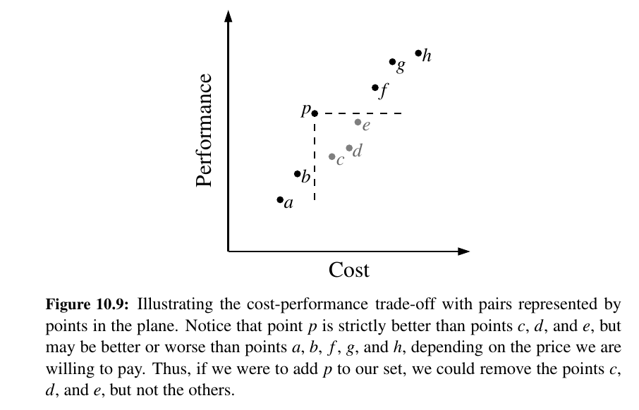
Maxima Sets¶

Life is full of trade-offs.

We often have to trade off a desired performance measure against a corresponding cost.

Suppose, for the sake of an example, we are interested in maintaining a database rating automobiles by their maximum speeds and their cost.

We would like to allow someone with a certain amount of money to query our database to find the fastest car they can possibly afford.

maxima_sets_from_real_world — A Maxima Set as a Car Evaluation Graph

TODO: Not urgent

...

Skip Lists¶

An interesting data structure for realizing the sorted map ADT is the skip list.

In Chapter 10.3.1, we saw that a sorted array will allow $O(log n)$-time searches via the binary search algorithm. Unfortunately, update operations on a sorted array have $O(n)$ worst-case running time because of the need to shift elements.

In Chapter 7 we demonstrated that linked lists support very efficient update operations, as long as the position within the list is identified. Unfortunately, we cannot perform fast searches on a standard linked list; for example, the binary search algorithm requires an efficient means for direct accessing an element of a sequence by index.

Skip lists provide a clever compromise to efficiently support search and update operations.

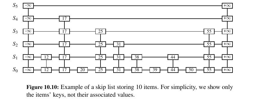
A skip list $S$ for a map $M$ consists of a series of lists ${S_0 , S_1 , . . . , S_h }$.

Each list $S_i$ stores a subset of the items of M sorted by increasing keys, plus items with two sentinel keys denoted −∞ and +∞, where −∞ is smaller than every possible key that can be inserted in M and +∞ is larger than every possible key that can be inserted in M.

In addition, the lists in S satisfy the following:

• List $S_0$ contains every item of the map M (plus sentinels −∞ and +∞).

• For $i = 1, . . . , h − 1,$ list $S_i$ contains (in addition to −∞ and +∞) a randomly generated subset of the items in list $S_{i−1}$ .

• List $S_h$ contains only −∞ and +∞.

TODO:

...

Search and Update Operations in a Skip List¶

TODO: Not urgent

...

Probabilistic Analysis of Skip Lists¶

TODO: Not urgent

...

Sets, Multisets, and Multimaps¶

We conclude this chapter by examining several additional abstractions that are closely related to the map ADT, and that can be implemented using data structures similar to those for a map.

• A set is an unordered collection of elements, without duplicates, that typically supports efficient membership tests. In essence, elements of a set are like keys of a map, but without any auxiliary values.

• A multiset (also known as a bag) is a set-like container that allows duplicates.

• A multimap is similar to a traditional map, in that it associates values with keys; however, in a multimap the same key can be mapped to multiple values. For example, the index of this book maps a given term to one or more locations at which the term occurs elsewhere in the book.

The Set ADT¶

Python provides support for representing the mathematical notion of a set through the built-in classes frozenset and set, as originally discussed in Chapter 1, with frozenset being an immutable form.

Both of those classes are implemented using hash tables in Python.

Here are the crucial methods of sets:

Method	Explanation
`S.add(e)`	Add element e to the set. This has no effect if the set already contains e.
`S.discard(e)`	Remove element e from the set, if present. This has ==no effect if the set does not contain e==.
`e in S`	Return True if the set contains element e. In Python, this is implemented with the special contains method.
`len(S)`	Return the number of elements in set S. In Python, this is implemented with the special method `__len__`
`iter(S)`	Generate an iteration of all elements of the set. In Python, this is implemented with the special method `__iter__` .
`S.remove(e)`	Remove element e from the set. If the set does not contain e, ==raise a== `KeyError`.
`S.pop()`	Remove and return an arbitrary element from the set. If the set is empty, raise a `KeyError`.
`S.clear()`	Remove all elements from the set.

The next group of behaviors perform Boolean comparisons between two sets.

Method	Explanation
`S == T`	Return True if sets S and T have identical contents.
`S != T`	Return True if sets S and T are not equivalent.
`S <= T`	Return True if set S is a subset of set T.
`S < T`	Return True if set S is a proper subset of set T.
`S >= T`	Return True if set S is a superset of set T.
`S > T`	Return True if set S is a proper superset of set T.
`S.isdisjoint(T)`	Return True if sets S and T have no common elements.

Finally, there exists a variety of behaviors that either update an existing set, or compute a new set instance, based on classical set theory operations.

Method	Explaination
`S \\| T`	Return a new set representing the union of sets S and T.
`S \\|= T`	Update set S to be the union of S and set T.
`S & T`	Return a new set representing the intersection of sets S and T.
`S &= T`	Update set S to be the intersection of S and set T.
`S ˆ T`	Return a new set representing the symmetric difference of sets S and T, that is, a set of elements that are in precisely one of S or T.
`S ˆ= T`	Update set S to become the symmetric difference of itself and set T.
`S − T`	Return a new set containing elements in S but not T.
`S −= T`	Update set S to remove all common elements with set T.

Python’s MutableSet Abstract Base Class¶

TODO: Not urgent

...

Implementing Sets, Multisets, and Multimaps¶

TODO: Not urgent

...

You are doing great!

Let's now discover Search Trees together. 💎

Operation	List	Hash Table Expected	Hash Table Worst
`__getitem__`	\(O(n)\)	\(O(1)\)	\(O(n)\)
`__setitem__`	\(O(n)\)	\(O(1)\)	\(O(n)\)
`__delitem__`	\(O(n)\)	\(O(1)\)	\(O(n)\)
`__len__`	\(O(1)\)	\(O(1)\)	\(O(1)\)
`__iter__`	\(O(n)\)	\(O(n)\)	\(O(n)\)

Maps, Hash Tables and Skip Lists¶

Maps and Dictionaries 😍¶

The Map ADT¶

Application: Counting Word Frequencies¶

Application: Finding The min/max Value based on values of dict¶

Python’s MutableMapping Abstract Base Class¶

Our MapBase Class¶

Simple Unsorted Map Implementation¶

Hash Tables¶

Hash Functions¶

Hash Codes¶

Treating the Bit Representation as an Integer¶

Polynomial Hash Codes¶

Cyclic-Shift Hash Codes¶

Hash Codes in Python 🥳¶

Compression Functions 😍¶

The Division Method¶

The MAD Method¶

Collision-Handling Schemes 🍒¶

Separate Chaining¶

Open Addressing¶

Linear Probing and Its Variants - Open Addressing Methods 💕¶

Quadratic Probing¶

Double Hashing 💖¶

Load Factors, Rehashing, and Efficiency 😯¶

Efficiency of Hash Tables 🤔¶

Python Hash Table Implementation¶

Separate Chaining Implementation¶

Linear Probing Implementation¶

Sorted Maps 🧡¶

Sorted Search Tables¶

Two Applications of Sorted Maps¶

Flight Databases¶

Maxima Sets¶

Skip Lists¶

Search and Update Operations in a Skip List¶

Probabilistic Analysis of Skip Lists¶

Sets, Multisets, and Multimaps¶

The Set ADT¶

Python’s MutableSet Abstract Base Class¶

Implementing Sets, Multisets, and Multimaps¶

Python’s `MutableMapping` Abstract Base Class¶

Our `MapBase` Class¶