Graphs 🥰

This chapter is all about graphs.

What is a Graph?

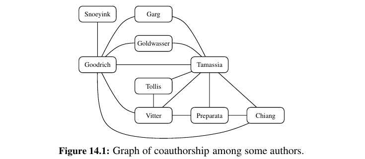
A graph G is simply a set V of vertices and a collection E of pairs of vertices from V, called edges.

Thus, a graph is a way of representing connections or relationships between pairs of objects from some set V.

A lot of definitions about them:

• Edges in a graph are either directed or undirected. An edge \((u, v)\) is said to be directed from \(u\) to \(v\) if the pair \((u, v)\) is ordered, with \(u\) preceding \(v\). An edge \((u, v)\) is said to be undirected if the pair \((u, v)\) is not ordered.

Graph if Authors

• If all the edges in a graph are undirected, then we say the graph is an undirected graph. Likewise, a directed graph, also called a digraph, is a graph whose edges are all directed. A graph that has both directed and undirected edges is often called a mixed graph.

• If an edge is directed, its first endpoint is its origin and the other is the destination of the edge.

• Two vertices u and v are said to be adjacent if there is an edge whose end vertices are u and v.

• An edge is said to be incident to a vertex if the vertex is one of the edge’s endpoints.

• The outgoing edges of a vertex are the directed edges whose origin is that vertex.

• The incoming edges of a vertex are the directed edges whose destination is that vertex.

• The degree of a vertex v, denoted deg(v), is the number of incident edges of v.

• The in-degree and out-degree of a vertex v are the number of the incoming and outgoing edges of v, and are denoted indeg(v) and outdeg(v) , respectively.

A flight network is a great example!

Flight Network

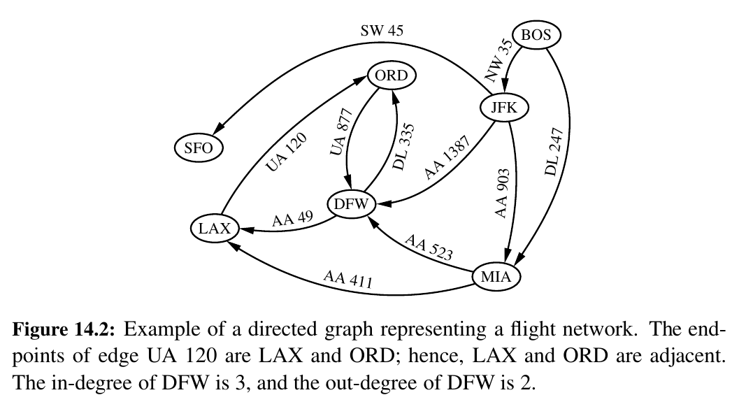
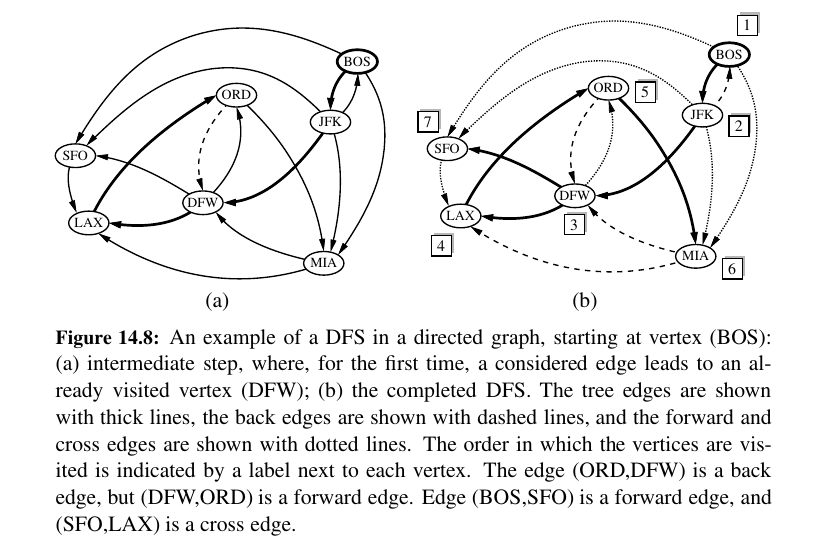
For example, DFW has out degree of 2 and in degree of 3.

The definition of a graph refers to the group of edges as a collection, not a set, thus allowing two undirected edges to have the same end vertices, and for two directed edges to have the same origin and the same destination. Such edges are called parallel edges or multiple edges.

A flight network can contain parallel edges, such that multiple edges between the same pair of vertices could indicate different flights operating on the same route at different times of the day.

Another special type of edge is one that connects a vertex to itself. Namely, we say that an edge (undirected or directed) is a self-loop if its two endpoints coincide.

With few exceptions, graphs do not have parallel edges or self-loops. Such graphs are said to be simple.

Assume simple unless otherwise specified.

A path is a sequence of alternating vertices and edges that starts at a vertex and ends at a vertex such that each edge is incident to its predecessor and successor vertex.

A cycle is a path that starts and ends at the same vertex, and that includes at least one edge.

We say that a path is simple if each vertex in the path is distinct, and we say that a cycle is simple if each vertex in the cycle is distinct, except for the first and last one.

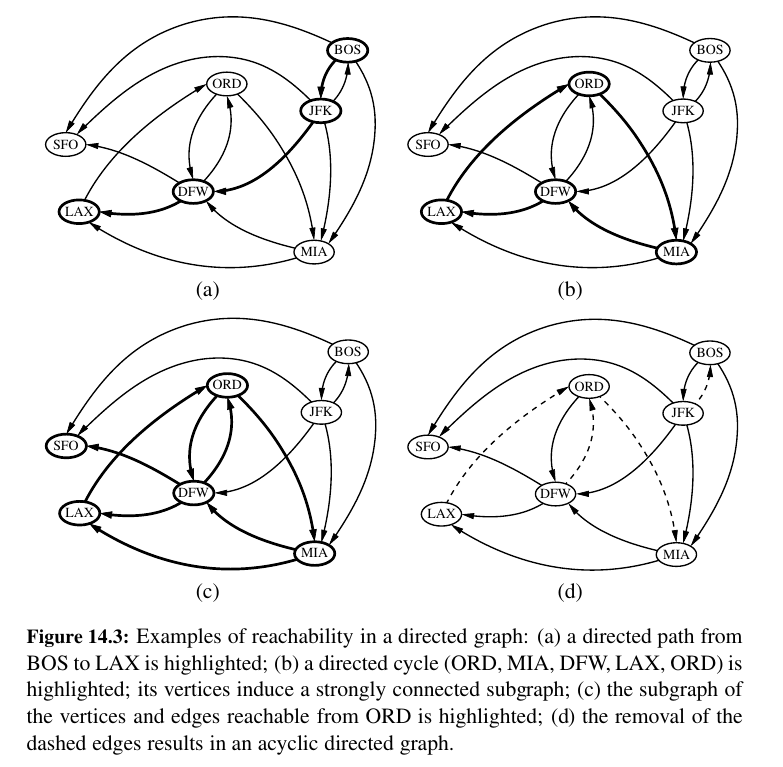
A directed path is a path such that all edges are directed and are traversed along their direction

For example, in Figure 14.2, (BOS, NW 35, JFK, AA 1387, DFW) is a directed simple path, and (LAX, UA 120, ORD, UA 877, DFW, AA 49, LAX) is a directed simple cycle.

Flight Network Again, to see paths and cycles

A directed graph is acyclic if it has no directed cycles.

Reachability in Directed Graph

In the propositions that follow, we explore a few important properties of graphs.

• If G is a graph with m edges and vertex set V , then: \(_{(v) in (V)}∑ deg(v) = 2m\)

• If G is a directed graph with m edges and vertex set V , then: \(_{(v) in (V)}∑ indeg(v) = _{(v) in (V)}∑ outdeg (v) = m\). Total in degree is equal to total out degree.

• Let G be an undirected graph with n vertices and m edges.

  • If G is connected, then m ≥ n − 1.

  • If G is a tree, then m = n − 1.

  • If G is a forest, then m ≤ n − 1.

The Graph ADT

TODO: Not urgent

...

Data Structures for Graphs 🥰

We will see four data structures for representing a graph.

In each representation, we maintain a collection to store the vertices of a graph.

However, the four representations differ greatly in the way they organize the edges.

• In an edge list, we maintain an unordered list of all edges. This minimally suffices, but there is no efficient way to locate a particular edge \((u, v)\), or the set of all edges incident to a vertex v.

• In an adjacency list, we maintain, for each vertex, a separate list containing those edges that are incident to the vertex. The complete set of edges can be determined by taking the union of the smaller sets, while the organization allows us to more efficiently find all edges incident to a given vertex.

• An adjacency map is very similar to an adjacency list, but the secondary container of all edges incident to a vertex is organized as a map, rather than as a list, with the adjacent vertex serving as a key. This allows for access to a specific edge \((u, v)\) in \(O(1)\) expected time.

• An adjacency matrix provides worst-case \(O(1)\) access to a specific edge \((u, v)\) by maintaining an n × n matrix, for a graph with n vertices. Each entry is dedicated to storing a reference to the edge \((u, v)\) for a particular pair of vertices u and v; if no such edge exists, the entry will be None. Uses a lot of memory.

Performance of these Data Structures for Graphs

Edge List Structure 💙

The edge list structure is possibly the simplest, though not the most efficient, representation of a graph G. All vertex objects are stored in an unordered list V, and all edge objects are stored in unordered list E.

Edge List Graph

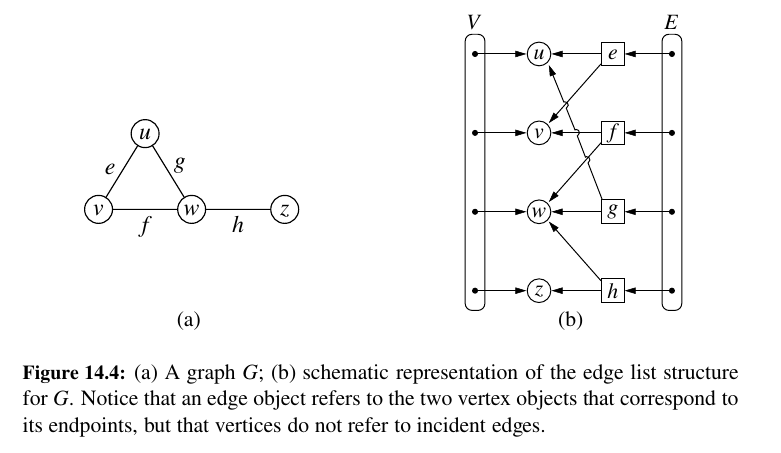
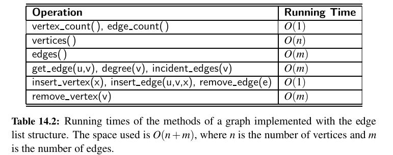
Performance:

The space usage, which is \(O(n + m)\) for representing a graph with n vertices and m edges.

The most significant limitations of an edge list structure, especially when compared to the other graph representations, are the \(O(m)\) running times of methods get_edge(u,v), degree(v), and incident_edges(v).

The problem is that with all edges of the graph in an unordered list E, the only way to answer those queries is through an exhaustive inspection of all edges.

The other data structures introduced in this section will implement these methods more efficiently.

Edge List Running Times

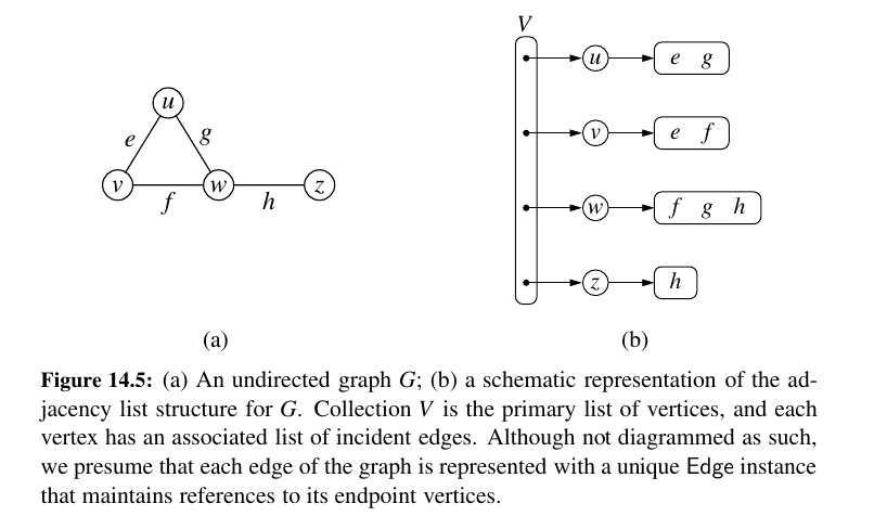
Adjacency List Structure 💚

In contrast to the edge list representation of a graph, the adjacency list structure groups the edges of a graph by storing them in smaller, secondary containers that are associated with each individual vertex.

Specifically, for each vertex v, we maintain a collection I(v), called the incidence collection of v, whose entries are edges incident to v.

In the case of a directed graph, outgoing and incoming edges can be respectively stored in two separate collections, \(I_{out}(v)\) and \(I_{in}(v)\).

Traditionally, the incidence collection I(v) for a vertex v is a list, which is why we call this way of representing a graph the adjacency list structure.

The primary benefit of an adjacency list is that the collection \(I(v)\) contains exactly those edges that should be reported by the method incident edges(v).

Therefore, we can implement this method by iterating the edges of \(I(v)\) in \(O(deg(v))\) time, where \(deg(v)\) is the degree of vertex v.

This is the best possible outcome for any graph representation, because there are \(deg(v)\) edges to be reported.

Adjacency List Graph

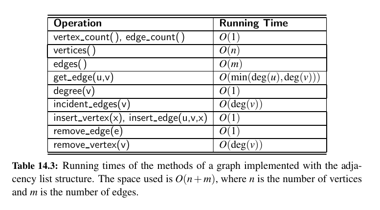
Performance:

Asymptotically, the space requirements for an adjacency list are the same as an edge list structure, using \(O(n + m)\) space for a graph with n vertices and m edges.

The primary list of vertices uses \(O(n)\) space. The sum of the lengths of all secondary lists is \(O(m)\), for reasons that were formalized in Propositions 14.8 and 14.9.

In short, an undirected edge (u, v) is referenced in both I(u) and I(v), but its presence in the graph results in only a constant amount of additional space.

We have already noted that the incident edges(v) method can be achieved in \(O(deg(v))\) time based on use of \(I(v)\).

We can achieve the degree(v) method of the graph ADT to use \(O(1)\) time, assuming collection \(I(v)\) can report its size in similar time.

To locate a specific edge for implementing get_edge(u,v), we can search through either I(u) and I(v). By choosing the smaller of the two, we get \(O(min(deg(u), deg(v)))\) running time.

Adjacency List Running Times

Adjacency Map Structure 💛

Expected \(o(1)\) time for edges. I think this is the one (Vertices as keys, edges as values)!

In the adjacency list structure, we assume that the secondary incidence collections are implemented as unordered linked lists.

Such a collection \(I(v)\) uses space proportional to \(O(deg(v))\), allows an edge to be added or removed in \(O(1)\) time, and allows an iteration of all edges incident to vertex v in \(O(deg(v))\) time.

However, the best implementation of get_edge(u,v) requires \(O(min(deg(u), deg(v)))\) time, because we must search through either \(I(u)\) or \(I(v)\).

We can improve the performance by using a hash-based map to implement I(v) for each vertex v.

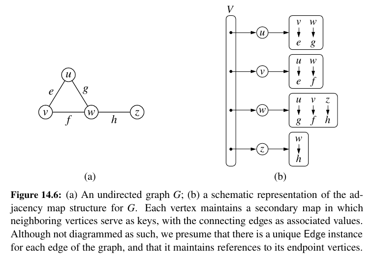
Specifically, we let the opposite endpoint of each incident edge serve as a key in the map, with the edge structure serving as the value.

We call such a graph representation an adjacency map. (See Figure 14.6.) The space usage for an adjacency map remains \(O(n + m)\), because I(v) uses \(O(deg(v))\) space for each vertex v, as with the adjacency list.

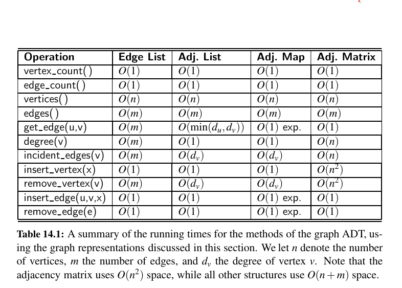
In comparing the performance of adjacency map to other representations (see Table 14.1), we find that it essentially achieves optimal running times for all methods, making it an excellent all-purpose choice as a graph representation.

Adjacency Map Graph

Adjacency Matrix Structure 🧡

\(O(1)\) worst case access FOR EDGES. Cool but lots of memory 😯 (Vertices as integers - edges being pairs of integers. Problem is adding and removing vertices. (resize matrix))

The adjacency matrix structure for a graph G augments the edge list structure with a matrix A (that is, a two-dimensional array, as in Chapter 5.6), which allows us to locate an edge between a given pair of vertices in worst-case constant time.

In the adjacency matrix representation, we think of the vertices as being the integers in the set \({0, 1, . . . , n − 1}\) and the edges as being pairs of such integers.

This allows us to store references to edges in the cells of a two-dimensional \(n × n\) array A.

The most significant advantage of an adjacency matrix is that any edge (u, v) can be accessed in worst-case \(O(1)\) time; recall that the adjacency map supports that operation in \(O(1)\) expected time.

However, several operation are less efficient with an adjacency matrix. For example, to find the edges incident to vertex v, we must presumably examine all n entries in the row associated with v; recall that an adjacency list or map can locate those edges in optimal \(O(deg(v))\) time.

Adding or removing vertices from a graph is problematic, as the matrix must be resized.

Furthermore, the \(O(n^2)\) space usage of an adjacency matrix is typically far worse than the \(O(n + m)\) space required of the other representations.

Although, in the worst case, the number of edges in a dense graph will be proportional to \(n^2\) , most real-world graphs are sparse.

Adjacency Matrix Graph

Python Implementation

For each vertex v, we use a Python dictionary to represent the secondary incidence map \(I(v)\).

However, we do not explicitly maintain lists V and E, as originally described in the edge list representation.

The list V is replaced by a top-level dictionary D that maps each vertex v to its incidence map \(I(v)\); note that we can iterate through all vertices by generating the set of keys for dictionary D.

See the implementation with adjacency map.

class Graph:
    """Representation of a simple graph using an adjacency map."""

    # ------------------------- nested Vertex class -------------------------
    class Vertex:
        """Lightweight vertex structure for a graph."""
        __slots__ = '_element'

        def __init__(self, x):
            """Do not call constructor directly. Use Graph's insert_vertex(x)."""
            self._element = x

        def element(self):
            """Return element associated with this vertex."""
            return self._element

        def __hash__(self):  # will allow vertex to be a map/set key
            return hash(id(self))

        def __str__(self):
            return str(self._element)

    # ------------------------- nested Edge class -------------------------
    class Edge:
        """Lightweight edge structure for a graph.
        An edge has origin destination element"""
        __slots__ = '_origin', '_destination', '_element'

        def __init__(self, u, v, x):
            """Do not call constructor directly. Use Graph's insert_edge(u,v,x)."""
            self._origin = u
            self._destination = v
            self._element = x

        def endpoints(self):
            """Return (u,v) tuple for vertices u and v."""
            return (self._origin, self._destination)

        def opposite(self, v):
            """Return the vertex that is opposite v on this edge."""
            if not isinstance(v, Graph.Vertex):
                raise TypeError('v must be a Vertex')
            return self._destination if v is self._origin else self._origin
            raise ValueError('v not incident to edge')

        def element(self):
            """Return element associated with this edge."""
            return self._element

        def __hash__(self):  # will allow edge to be a map/set key
            """Hash the Tuple!"""
            return hash((self._origin, self._destination))

        def __str__(self):
            return '({0},{1},{2})'.format(self._origin, self._destination, self._element)

    # ------------------------- Graph methods -------------------------
    def __init__(self, directed=False):
        """Create an empty graph (undirected, by default).
        Graph is directed if optional paramter is set to True.
        """
        # this is our adjecancy map
        self._outgoing = {}
        # only create second map for directed graph; use alias for undirected
        self._incoming = {} if directed else self._outgoing

    def _validate_vertex(self, v):
        """Verify that v is a Vertex of this graph."""
        if not isinstance(v, self.Vertex):
            raise TypeError('Vertex expected')
        if v not in self._outgoing:
            raise ValueError('Vertex does not belong to this graph.')

    def is_directed(self):
        """Return True if this is a directed graph; False if undirected.
        Property is based on the original declaration of the graph, not its contents.
        """
        return self._incoming is not self._outgoing  # directed if maps are distinct

    def vertex_count(self):
        """Return the number of vertices in the graph."""
        return len(self._outgoing)

    def vertices(self):
        """Return an iteration of all vertices of the graph."""
        return self._outgoing.keys()

    def edge_count(self):
        """Return the number of edges in the graph."""
        #                edges                    all keys (vertices)
        total = sum(len(self._outgoing[v]) for v in self._outgoing)
        # for undirected graphs, make sure not to double-count edges
        return total if self.is_directed() else total // 2

    def edges(self):
        """Return a set of all edges of the graph."""
        result = set()  # avoid double-reporting edges of undirected graph
        for secondary_map in self._outgoing.values():
            result.update(secondary_map.values())  # add edges to resulting set
        return result

    def get_edge(self, u, v):
        """Return the edge from u to v, or None if not adjacent."""
        self._validate_vertex(u)
        self._validate_vertex(v)
        return self._outgoing[u].get(v)  # returns None if v not adjacent

    def degree(self, v, outgoing=True):
        """Return number of (outgoing) edges incident to vertex v in the graph.
        If graph is directed, optional parameter used to count incoming edges.
        """
        self._validate_vertex(v)
        # change behaviour on parameter!
        adj = self._outgoing if outgoing else self._incoming
        return len(adj[v])

    def incident_edges(self, v, outgoing=True):
        """Return all (outgoing) edges incident to vertex v in the graph.
        If graph is directed, optional parameter used to request incoming edges.
        """
        self._validate_vertex(v)
        adj = self._outgoing if outgoing else self._incoming
        for edge in adj[v].values():
            yield edge

    def insert_vertex(self, x=None):
        """Insert and return a new Vertex with element x."""
        v = self.Vertex(x)
        self._outgoing[v] = {}
        if self.is_directed():
            self._incoming[v] = {}  # need distinct map for incoming edges
        return v

    def insert_edge(self, u, v, x=None):
        """Insert and return a new Edge from u to v with auxiliary element x.
        Raise a ValueError if u and v are not vertices of the graph.
        Raise a ValueError if u and v are already adjacent.
        """
        if self.get_edge(u, v) is not None:  # includes error checking
            raise ValueError('u and v are already adjacent')
        e = self.Edge(u, v, x)
        self._outgoing[u][v] = e
        self._incoming[v][u] = e

Graphs in Real World:

Here is a typical interview question.

Given an m x n 2D binary grid grid which represents a map of '1's (land) and '0's (water), return the number of islands.

An island is surrounded by water and is formed by connecting adjacent lands horizontally or vertically. You may assume all four edges of the grid are all surrounded by water.

Example 1:

Input: grid = [
  ["1","1","1","1","0"],
  ["1","1","0","1","0"],
  ["1","1","0","0","0"],
  ["0","0","0","0","0"]
]
Output: 1

Example 2:

Input: grid = [
  ["1","1","0","0","0"],
  ["1","1","0","0","0"],
  ["0","0","1","0","0"],
  ["0","0","0","1","1"]
]
Output: 3

Constraints:

m == grid.length
n == grid[i].length
1 <= m, n <= 300
grid[i][j] is '0' or '1'.

class Solution:

    def numIslands(self, grid: list[list[str]]) -> int:
        m = len(grid)
        n = len(grid[0])
        result = 0

        def dfs(i, j):
            if (i < 0 or 
                j < 0 or 
                i >= m or 
                j >= n or 
                grid[i][j] == '0'):
                    return
            # make the current tile 0
            # so you will not count this tile again
            grid[i][j] = '0'

            # go to every direction possible
            dfs(i - 1, j)
            dfs(i + 1, j)
            dfs(i, j - 1)
            dfs(i, j + 1)

        for i in range(m):
            for j in range(n):
                if grid[i][j] == '1':
                    result += 1
                    dfs(i, j)

        return result

Graph Traversals 💗

A traversal is a systematic procedure for exploring a graph by examining all of its vertices and edges.

A traversal is efficient if it visits all the vertices and edges in time proportional to their number, that is, in linear time.

Graph traversal algorithms are key to answering many fundamental questions about graphs involving the notion of reachability, that is, in determining how to travel from one vertex to another while following paths of a graph.

• Problems to deal with reachability for undirected graphs:

  • Computing a path from vertex u to vertex v, or reporting that no such path exists.

  • Given a start vertex s of G, computing, for every vertex v of G, a path with the minimum number of edges between s and v, or reporting that no such path exists.

  • Testing whether G is connected.

  • Computing a spanning tree of G, if G is connected.

  • Computing the connected components of G.

  • Computing a cycle in G, or reporting that G has no cycles.

• Problems to deal with reachability for directed graphs:

  • Computing a directed path from vertex u to vertex v, or reporting that no such path exists.

  • Finding all the vertices of \(\vec{G}\) that are reachable from a given vertex s.

  • Determine whether \(\vec{G}\) is acyclic.

  • Determine whether \(\vec{G}\) is strongly connected.

DFS

Depth-first search (DFS) is an algorithm for traversing or searching tree or graph data structures.

Wisdom: Sending single agent with a rope in a labyrinth. We go as deep as possible, we backtrack from dead ends.

Algorithm DFS(G,u):      {We assume u has already been marked as visited}
    Input: A graph G and a vertex u of G
    Output: A collection of vertices reachable from u, with their discovery edges
        for each outgoing edge e = (u, v) of u do
            if vertex v has not been visited then
                Mark vertex v as visited (via edge e).
                Recursively call DFS(G,v).

Here is DFS on directed graph:

DFS on Directed Graph

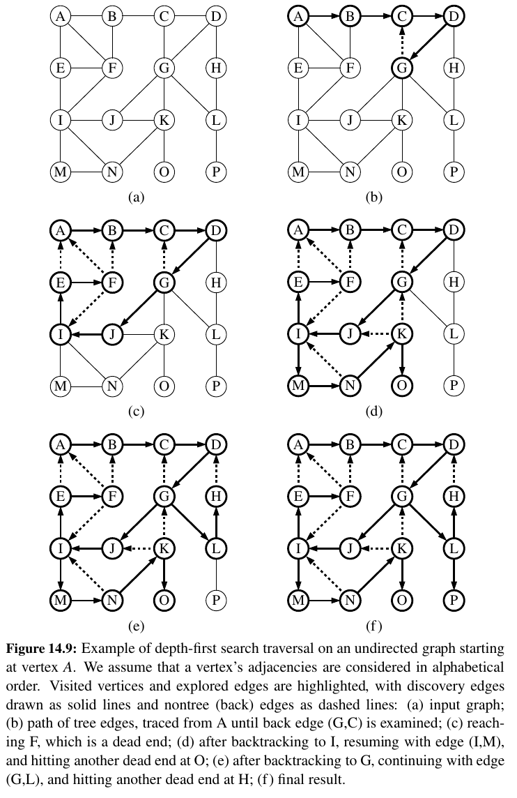
Here is DFS on undirected graph (full arrows are discovery, dotted arrows are back edges):

DFS on Undirected Graph

Properties of DFS

Proposition 14.12: Let G be an undirected graph on which a DFS traversal starting at a vertex s has been performed. Then the traversal visits all vertices in the connected component of s, and the discovery edges form a spanning tree of the connected component of s.

Depth-first search visits each vertex in the connected component of s.

For \(\vec{G}\) DFS visits all reachable.

Running time of DFS

For DFS, every edge is examined at most twice.

In terms of its running time, depth-first search is an efficient method for traversing a graph.

Note that DFS is called at most once on each vertex (since it gets marked as visited), and therefore every edge is examined at most twice for an undirected graph, once from each of its end vertices, and at most once in a directed graph, from its origin vertex.

When is it good too use DFS?

Proposition 14.14: Let G be an undirected graph with n vertices and m edges.

A DFS traversal of G can be performed in \(O(n + m)\) time, and can be used to solve the following problems in \(O(n + m)\) time:

• Computing a path between two given vertices of G, if one exists.

• Testing whether G is connected.

• Computing a spanning tree of G, if G is connected.

• Computing the connected components of G.

• Computing a cycle in G, or reporting that G has no cycles.

Proposition 14.15: Let \(\vec{G}\) be a directed graph with n vertices and m edges.

A DFS traversal of \(\vec{G}\) can be performed in \(O(n + m)\) time, and can be used to solve the following problems in \(O(n + m)\) time:

• Computing a directed path between two given vertices of \(\vec{G}\), if one exists.

• Computing the set of vertices of \(\vec{G}\) that are reachable from a given vertex s.

• Testing whether \(\vec{G}\) is strongly connected.

• Computing a directed cycle in \(\vec{G}\), or reporting that \(\vec{G}\) is acyclic.

• Computing the transitive closure of \(\vec{G}\) (see Section 14.4).

Tip

In real world we use set() for visited nodes while traversing.

BFS

Breadth First Search (BFS) is another fundamental graph traversal algorithm.

In this section, we consider another algorithm for traversing a connected component of a graph, known as a breadth-first search (BFS).

The BFS algorithm is more akin to sending out, in all directions, many explorers who collectively traverse a graph in coordinated fashion.

def BFS(g, s, discovered):
    """Perform BFS of the undiscovered portion of Graph g starting at Vertex s.
    discovered is a dictionary mapping each vertex to the edge that was used to
    discover it during the BFS (s should be mapped to None prior to the call).
    Newly discovered vertices will be added to the dictionary as a result.
    """
    level = [s]  # first level includes only s
    while len(level) > 0:
        next_level = []  # prepare to gather newly found vertices
        for u in level:
            for e in g.incident_edges(u):  # for every outgoing edge from u
                v = e.opposite(u)
                if v not in discovered:  # v is an unvisited vertex
                    discovered[v] = e  # e is the tree edge that discovered v
                    next_level.append(v)  # v will be further considered in next pass
        level = next_level  # relabel 'next' level to become current

BFS Example

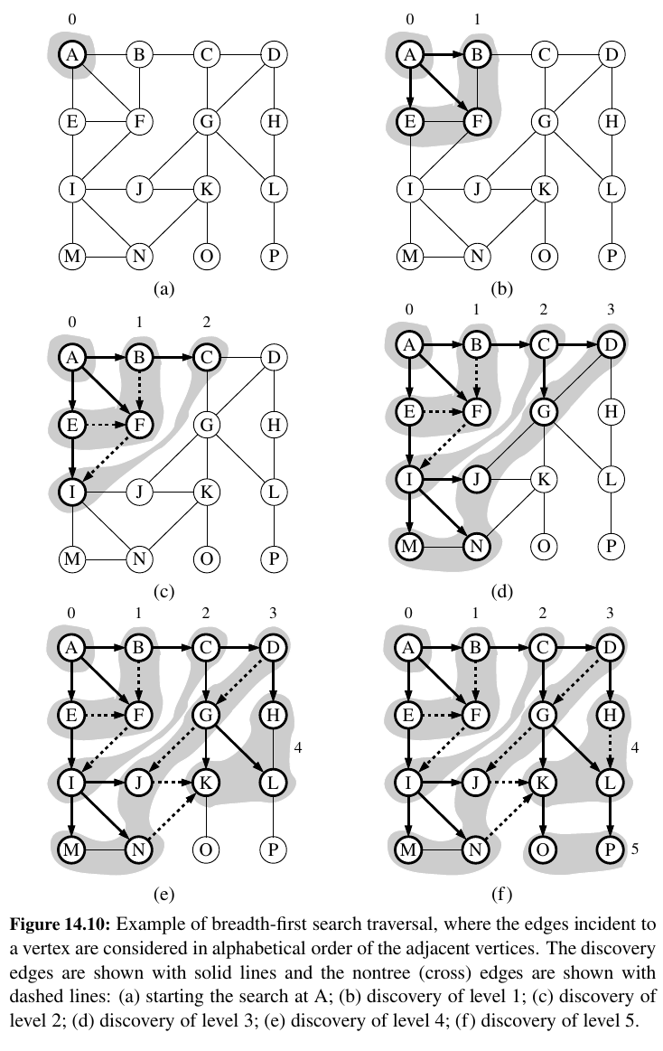
• A path in a breadth-first search tree rooted at vertex s to any other vertex v is guaranteed to be the shortest such path from s to v in terms of the number of edges.

Proposition 14.16: Let G be an undirected or directed graph on which a BFS traversal starting at vertex s has been performed.

Then

• The traversal visits all vertices of G that are reachable from s.

• For each vertex v at level i, the path of the BFS tree T between s and v has i edges, and any other path of G from s to v has at least i edges.

• If \((u, v)\) is an edge that is not in the BFS tree, then the level number of v can be at most 1 greater than the level number of u.

Let G be a graph with n vertices and m edges represented with the adjacency list structure. A BFS traversal of G takes \(O(n + m)\) time.

Transitive Closure

We have seen that graph traversals can be used to answer basic questions of reachability in a directed graph.

If representing a graph with an adjacency list or adjacency map, we can answer the question of reachability for u and v in \(O(n + m)\) time.

In an electricity network, we may wish to be able to quickly determine whether current flows from one particular vertex to another. Motivated by such applications, we introduce the following definition.

The transitive closure of a directed graph \(\vec{G}\) is itself a directed graph \(\vec{G}\)∗ such that the vertices of \(\vec{G}\)∗ are the same as the vertices of \(\vec{G}\), and \(\vec{G}\)∗ has an edge (u, v), whenever \(\vec{G}\) has a directed path from u to v (including the case where (u, v) is an edge of the original \(\vec{G}\)).

Transitive Closure

From vertice \(V\) where can I go?

TODO: Not urgent

...

Directed Acyclic Graphs

Directed graphs without directed cycles are encountered in many applications.

Such a directed graph is often referred to as a directed acyclic graph, or DAG, for short.

Applications of such graphs include the following:

• Prerequisites between courses of a degree program.

• Inheritance between classes of an object-oriented program.

• Scheduling constraints between the tasks of a project.

A great example would be Apache Airflow!

Directed Acyclic Graphs

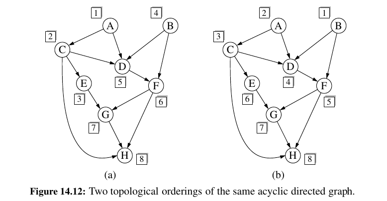
Topological Sorting ?

TODO: Not urgent

...

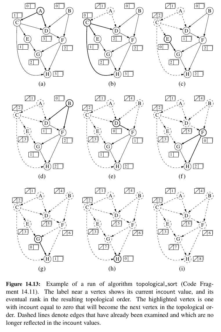
Just code:

def topological_sort(g):
    """Return a list of verticies of directed acyclic graph g in topological order.
    If graph g has a cycle, the result will be incomplete.
    """
    topo = []  # a list of vertices placed in topological order
    ready = []  # list of vertices that have no remaining constraints
    incount = {}  # keep track of in-degree for each vertex
    for u in g.vertices():
        incount[u] = g.degree(u, False)  # parameter requests incoming degree
        if incount[u] == 0:  # if u has no incoming edges,
            ready.append(u)  # it is free of constraints
    while len(ready) > 0:
        u = ready.pop()  # u is free of constraints
        topo.append(u)  # add u to the topological order
        for e in g.incident_edges(u):  # consider all outgoing neighbors of u
            v = e.opposite(u)
            incount[v] -= 1  # v has one less constraint without u
            if incount[v] == 0:
                ready.append(v)
    return topo

Example Run for Topological Sort

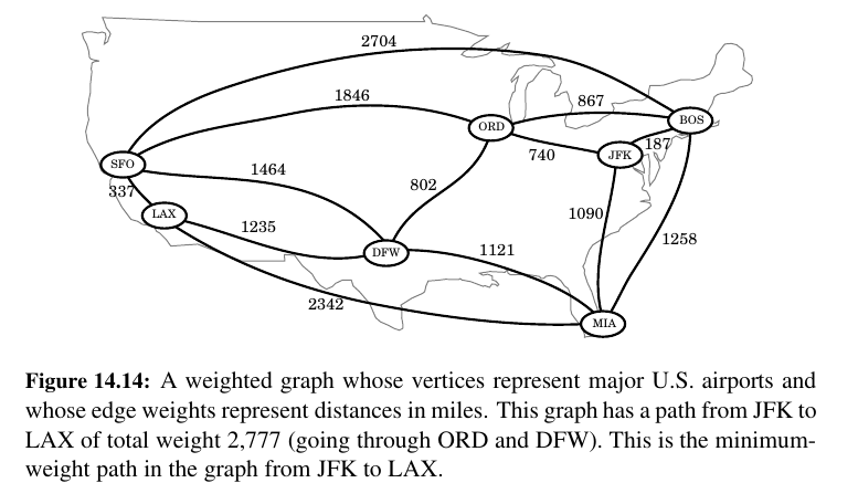
Shortest Paths

Some edges are better than others.

We might want to use a graph to represent the roads between cities, and we might be interested in finding the fastest way to travel cross-country.

In this case, it is probably not appropriate for all the edges to be equal to each other, for some inter-city distances will likely be much larger than others.

Weighted Graphs

A weighted graph is a graph that has a numeric (for example, integer) label \(w(e)\) associated with each edge \(e\), called the weight of edge \(e\). For \(e = (u, v)\), we let notation \(w(u, v) = w(e)\)

Weighted Graphs

If there is a negative weight (ORD - 70 JFK: someone paying us to go to JFK) that would be infinite money glitch 😅

If the special case of computing a shortest path when all weights are equal to one was solved with the BFS traversal algorithm.

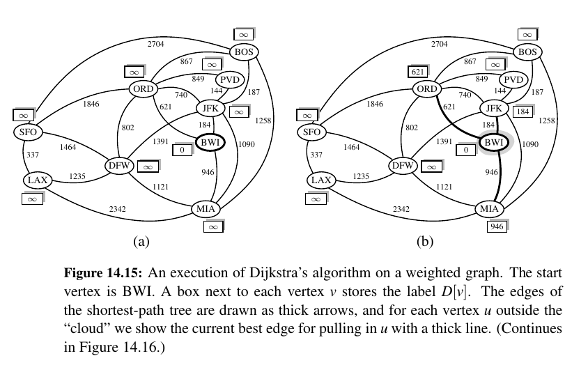
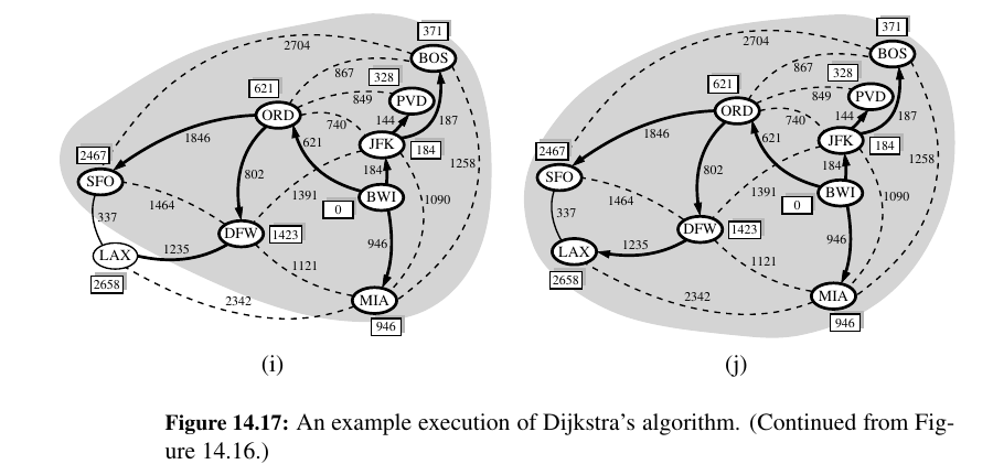
Dijkstra's Algorithm 🥳

The main idea in applying the greedy method pattern to the single-source shortest-path problem is to perform a “weighted” breadth-first search starting at the source vertex s.

In particular, we can use the greedy method to develop an algorithm that iteratively grows a “cloud” of vertices out of s, with the vertices entering the cloud in order of their distances from s.

Thus, in each iteration, the next vertex chosen is the vertex outside the cloud that is closest to s.

The algorithm terminates when no more vertices are outside the cloud (or when those outside the cloud are not connected to those within the cloud), at which point we have a shortest path from s to every vertex of G that is reachable from s.

This approach is a simple, but nevertheless powerful, example of the greedy method design pattern. Applying the greedy method to the single-source, shortest-path problem, results in an algorithm known as Dijkstra’s algorithm.

Once a new vertex u is pulled into C, we then update the label D[v] of each vertex v that is adjacent to u and is outside of C, to reflect the fact that there may be a new and better way to get to v via u.

This update operation is known as a relaxation procedure, for it takes an old estimate and checks if it can be improved to get closer to its true value.

Algorithm ShortestPath(G, s):
Input: A weighted graph G with nonnegative edge weights, and a distinguished vertex s of G.
Output: The length of a shortest path from s to v for each vertex v of G.
    Initialize D[s] = 0 and D[v] = ∞ for each vertex v != s.
    Let a priority queue Q contain all the vertices of G using the D labels as keys.
    while Q is not empty do
        {pull a new vertex u into the cloud}
        u = value returned by Q.remove min()
        for each vertex v adjacent to u such that v is in Q do
            {perform the relaxation procedure on edge (u, v)}
            if D[u] + w(u, v) < D[v] then
                D[v] = D[u] + w(u, v)
                Change to D[v] the key of vertex v in Q.
    return the label D[v] of each vertex v

Dijkstra on a Weighted Graph

Stage f - we find a new better path. ORD -> DFW 1423 (802 - 621)

Dijkstra on a Weighted Graph Continued

Dijkstra on a Weighted Graph End

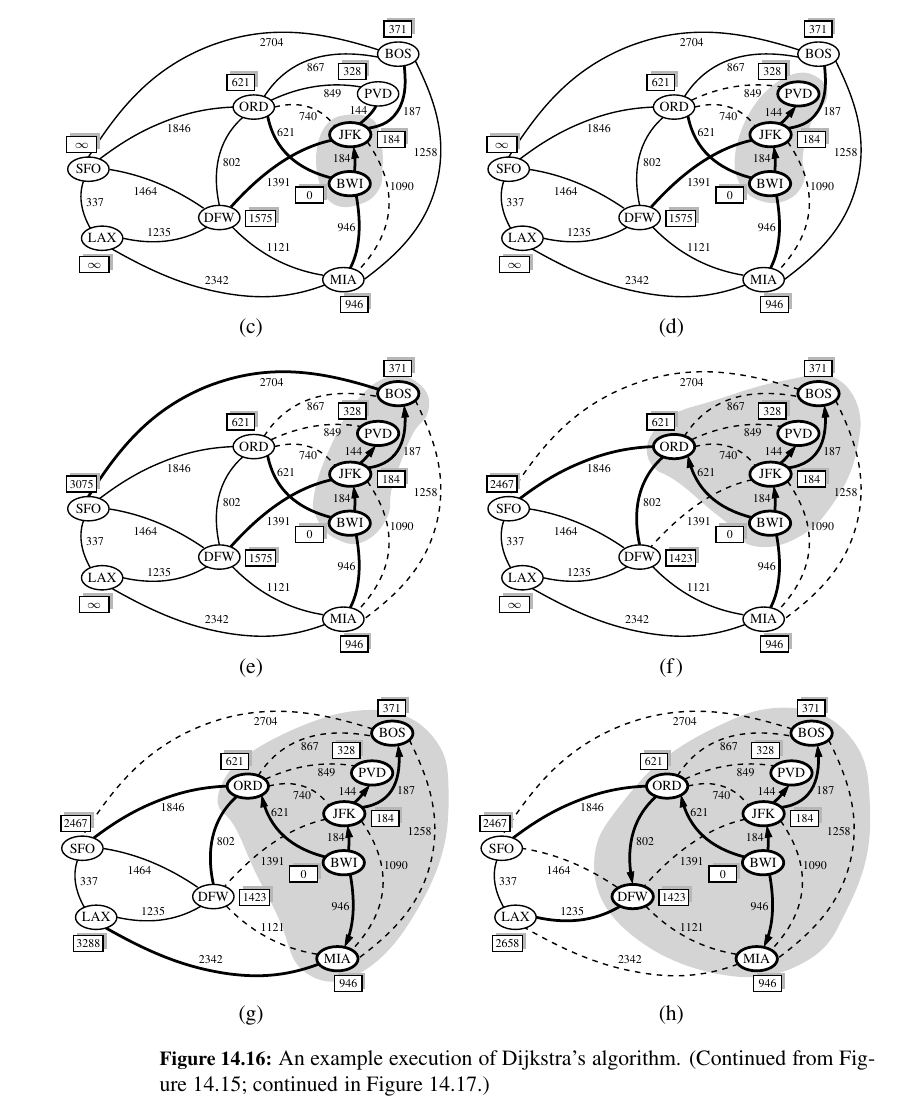
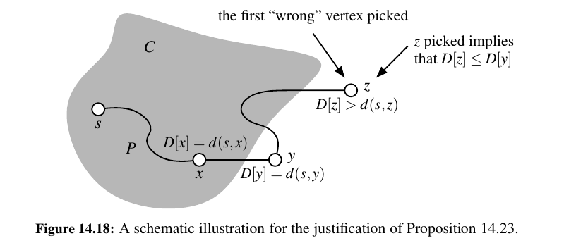
The answer to this question depends on there being no negative-weight edges in the graph, for it allows the greedy method to work correctly, as we show in the proposition that follows.

Proposition 14.23: In Dijkstra’s algorithm, whenever a vertex v is pulled into the cloud, the label D[v] is equal to d(s, v), the length of a shortest path from s to v.

Justification for Proposition 14.23

Running Time of Dijkstra

Let us first assume that we are representing the graph G using an adjacency list or adjacency map structure.

The outer while loop executes O(n) times, since a new vertex is added to the cloud during each iteration

It works with an adaptable Priority Queue and a unsorted list.

Overall, the running time of Dijkstra’s algorithm is bounded by the sum of the following:

• n insertions into Q.

• n calls to the remove min method on Q.

• m calls to the update method on Q.

If Q is an adaptable priority queue implemented as a heap, then each of the above operations run in O(log n), and so the overall running time for Dijkstra’s algorithm is \(O((n + m) log n)\).

Note that if we wish to express the running time as a function of n only, then it is \(O(n^{2} * log n)\) in the worst case.

Assuming we are given a graph whose edge elements are non negative integer weights.

Here is the code for Dijkstra:

def shortest_path_lengths(g, src):
    """Compute shortest-path distances from src to reachable vertices of g.
    Graph g can be undirected or directed, but must be weighted such that
    e.element() returns a numeric weight for each edge e.
    Return dictionary mapping each reachable vertex to its distance from src.
    """
    d = {}  # d[v] is upper bound from s to v
    cloud = {}  # map reachable v to its d[v] value
    pq = AdaptableHeapPriorityQueue()  # vertex v will have key d[v]
    pqlocator = {}  # map from vertex to its pq locator
    # for each vertex v of the graph, add an entry to the priority queue, with
    # the source having distance 0 and all others having infinite distance
    for v in g.vertices():
        if v is src:
            d[v] = 0
        else:
            d[v] = float('inf')  # syntax for positive infinity
        pqlocator[v] = pq.add(d[v], v)  # save locator for future updates
    while not pq.is_empty():
        key, u = pq.remove_min()
        cloud[u] = key  # its correct d[u] value
        del pqlocator[u]  # u is no longer in pq
        for e in g.incident_edges(u):  # outgoing edges (u,v)
            v = e.opposite(u)
            if v not in cloud:
                # perform relaxation step on edge (u,v)
                wgt = e.element()
                if d[u] + wgt < d[v]:  # better path to v?
                    d[v] = d[u] + wgt  # update the distance
                    pq.update(pqlocator[v], d[v], v)  # update the pq entry
    return cloud  # only includes reachable vertices

Shortest Path Tree

The collection of all shortest paths emanating from source s can be compactly represented by what is known as the shortest-path tree.

The paths form a rooted tree because if a shortest path from s to v passes through an intermediate vertex u, it must begin with a shortest path from s to u.

In this section, we demonstrate that the shortest-path tree rooted at source s can be reconstructed in \(O(n + m)\) time, given the set of d[v] values produced by Dijkstra’s algorithm using s as the source.

Here is the Python function that reconstructs the shortest paths, based on knowledge of the single-source distances:

def shortest_path_tree(g, s, d):
    """Reconstruct shortest-path tree rooted at vertex s, given distance map d.
    Return tree as a map from each reachable vertex v (other than s) to the
    edge e=(u,v) that is used to reach v from its parent u in the tree.
    """
    tree = {}
    for v in d:
        if v is not s:
            for e in g.incident_edges(v, False):  # consider INCOMING edges
                u = e.opposite(v)
                wgt = e.element()
                if d[v] == d[u] + wgt:
                    tree[v] = e  # edge e is used to reach v
    return tree

Minimum Spanning Trees

What if our goal was to find the tree T that contains all vertices of G and has min total Weight.

MST - Minimum spanning Trees

2 WAYS

TODO: not urgent

...

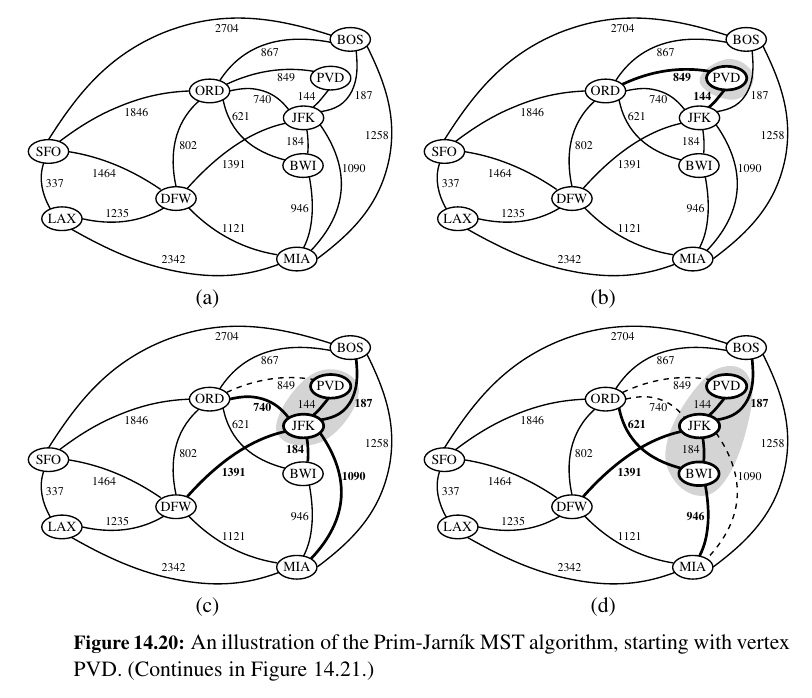
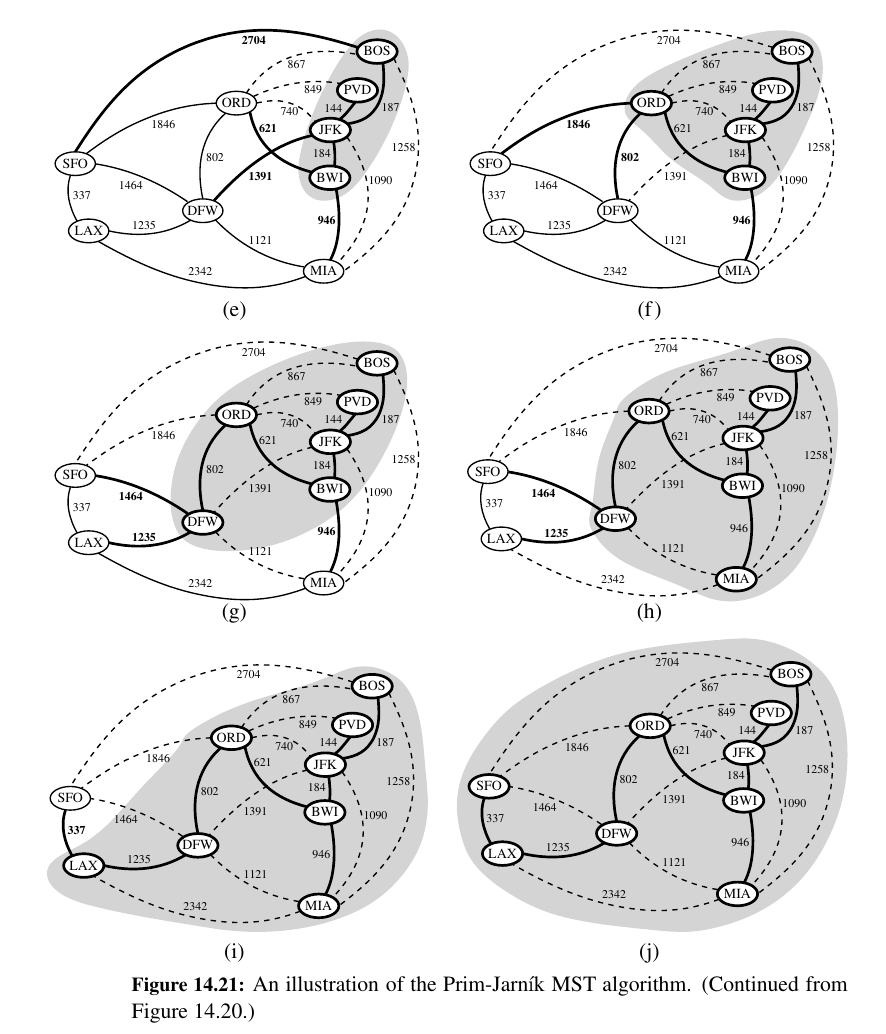
Prim Jarnik Algorithm

Make a single tree like Dijkstra.

In the Prim-Jarnı́k algorithm, we grow a minimum spanning tree from a single cluster starting from some “root” vertex s.

The main idea is similar to that of Dijkstra’s algorithm.

We begin with some vertex s, defining the initial “cloud” of vertices C. Then, in each iteration, we choose a minimum-weight edge e = (u, v), connecting a vertex u in the cloud C to a vertex v outside of C.

The vertex v is then brought into the cloud C and the process is repeated until a spanning tree is formed.

Again, the crucial fact about minimum spanning trees comes into play, for by always choosing the smallest-weight edge joining a vertex inside C to one outside C, we are assured of always adding a valid edge to the MST.

Prim Jarnik Start

Prim Jarnik End

Here is Python implementation of the Prim-Jarnı́k algorithm for the minimum spanning tree problem:

def MST_PrimJarnik(g):
    """Compute a minimum spanning tree of weighted graph g.
    Return a list of edges that comprise the MST (in arbitrary order).
    """
    d = {}  # d[v] is bound on distance to tree
    tree = []  # list of edges in spanning tree
    pq = AdaptableHeapPriorityQueue()  # d[v] maps to value (v, e=(u,v))
    pqlocator = {}  # map from vertex to its pq locator
    # for each vertex v of the graph, add an entry to the priority queue, with
    # the source having distance 0 and all others having infinite distance
    for v in g.vertices():
        if len(d) == 0:  # this is the first node
            d[v] = 0  # make it the root
        else:
            d[v] = float('inf')  # positive infinity
        pqlocator[v] = pq.add(d[v], (v, None))
    while not pq.is_empty():
        key, value = pq.remove_min()
        u, edge = value  # unpack tuple from pq
        del pqlocator[u]  # u is no longer in pq
        if edge is not None:
            tree.append(edge)  # add edge to tree
        for link in g.incident_edges(u):
            v = link.opposite(u)
            if v in pqlocator:  # thus v not yet in tree
                # see if edge (u,v) better connects v to the growing tree
                wgt = link.element()
                if wgt < d[v]:  # better edge to v?
                    d[v] = wgt  # update the distance
                    pq.update(pqlocator[v], d[v], (v, link))  # update the pq entry
    return tree

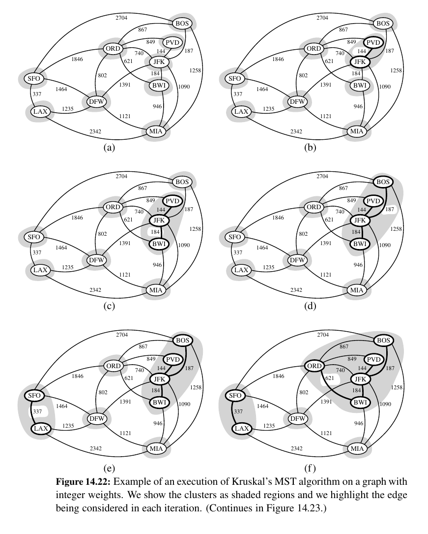
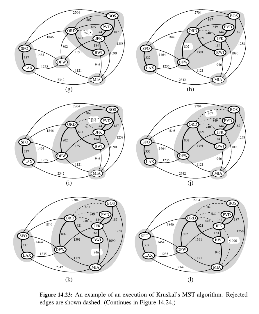
Kruskal's Algorithm

Make a forest , make discards and merges if needed UNTIL you find the ADEQUATELY BIG tree.

Here is the Pseudo code:

Algorithm Kruskal(G):
    Input: A simple connected weighted graph G with n vertices and m edges
    Output: A minimum spanning tree T for G
    for each vertex v in G do
        Define an elementary cluster C(v) = {v}.
    Initialize a priority queue Q to contain all edges in G, using the weights as keys.
    T = ∅                              {T will ultimately contain the edges of the MST}
    while T has fewer than n − 1 edges do
        (u, v) = value returned by Q.remove min()
        Let C(u) be the cluster containing u, and let C(v) be the cluster containing v.
        if C(u) = C(v) then
            Add edge (u, v) to T .
            Merge C(u) and C(v) into one cluster.
    return tree T

Kruskal on a Weighted Graph Start

Kruskal on a Weighted Graph Continued

Kruskal on a Weighted Graph End

The Running Time of Kruskal’s Algorithm

There are two primary contributions to the running time of Kruskal’s algorithm.

The first is the need to consider the edges in non decreasing order of their weights, and the second is the management of the cluster partition.

Analyzing its running time requires that we give more details on its implementation.

Here is Python implementation of Kruskal’s algorithm for the minimum spanning tree problem:

def MST_Kruskal(g):
    """Compute a minimum spanning tree of a graph using Kruskal's algorithm.
    Return a list of edges that comprise the MST.
    The elements of the graph's edges are assumed to be weights.
    """
    tree = []  # list of edges in spanning tree
    pq = HeapPriorityQueue()  # entries are edges in G, with weights as key
    forest = Partition()  # keeps track of forest clusters
    position = {}  # map each node to its Partition entry
    for v in g.vertices():
        position[v] = forest.make_group(v)
    for e in g.edges():
        pq.add(e.element(), e)  # edge's element is assumed to be its weight
    size = g.vertex_count()
    while len(tree) != size - 1 and not pq.is_empty():
        # tree not spanning and unprocessed edges remain
        weight, edge = pq.remove_min()
        u, v = edge.endpoints()
        a = forest.find(position[u])
        b = forest.find(position[v])
        if a != b:
            tree.append(edge)
            forest.union(a, b)
    return tree

Disjoint Partitions and Union-Find Structures

TODO , not urgent

...

On to the last chapter, Memory Management and B-Trees 💕