Algorithm Analysis 🏂¶

In this book, we are interested in the design of “good” data structures and algorithms.

Simply put, a data structure is a systematic way of organizing and accessing data and an algorithm is a step-by-step procedure for performing some task in a finite amount of time.

These concepts are central to computing, but to be able to classify some data structures and algorithms as “good” we must have precise ways of analyzing them.

Before you continue, do not forget that there is absolutely value in using time.perf_counter_ns() on a running code. You can understand where the code is spending it's time the most and make changes on it to see the effects after.

Experimental Studies¶

If an algorithm has been implemented, we can study its running time by executing it on various test inputs and recording the time spent during each execution.

Most basic way is using time. This is not good because at the time we test, the CPU might be loaded so it is not fair/reliable.

We can use CPU cycles, which is a bit better. Even this might not be consistent if repeated on identical algorithm with an identical input.

Most advanced one is Python's timeit module.

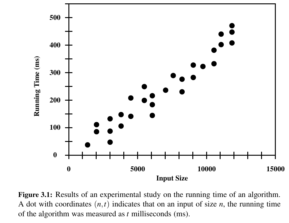
But there are some challenges to experimental analysis:

• Experimental running times of two algorithms are difficult to directly compare unless the experiments are performed in the same hardware and software environments. 😕

• Experiments can be done only on a limited set of test inputs; hence, they leave out the running times of inputs not included in the experiment (and these inputs may be important). 😕

• Algorithm must be fully implemented in order to execute it to study its running time experimentally. 😕

Moving beyond experimental analysis? 🤔¶

Is there something independent of OS, takes into account of all possible inputs and with a high level description (without the need of implementation) ?

Counting Primitive Operations¶

To analyze the running time of an algorithm without performing experiments, we perform an analysis directly on a high-level description of the algorithm (either in the form of an actual code fragment, or language-independent pseudo-code).

We define a set of primitive operations such as the following:

Assigning an identifier to an object
Determining the object associated with an identifier
Performing an arithmetic operation (for example, adding two numbers)
Comparing two numbers
Accessing a single element of a Python list by index
Calling a function (excluding operations executed within the function)
Returning from a function.

This operation count will correlate to an actual running time in a specific computer, for each primitive operation corresponds to a constant number of instructions, and there are only a fixed number of primitive operations.

Measuring Operations as a Function of Input Size¶

To capture the order of growth of an algorithm’s running time, we will associate, with each algorithm, a function f(n) that characterizes the number of primitive operations that are performed as a function of the input size n.

So the f(n) is to characterize the number of primitive operations.

Focusing on the Worst Case Input¶

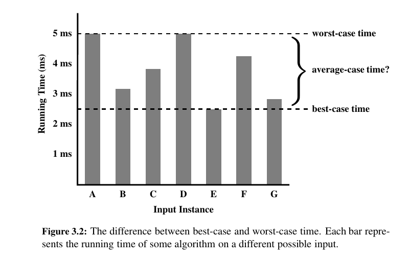
An algorithm may run faster on some inputs than it does on others of the same size.

Thus, we may wish to express the running time of an algorithm as the function of the input size obtained by taking the average over all possible inputs of the same size. Unfortunately, such an average-case analysis is typically quite challenging.

Worst-case analysis is much easier than average-case analysis, as it requires only the ability to identify the worst-case input, which is often simple.

That is, designing for the worst case leads to stronger algorithmic “muscles,” much like a track star who always practices by running up an incline.

Train with the weights on. 🏋️‍♂️

Seven Functions - `the 7` 😉¶

In this section, we briefly discuss the seven most important functions used in the analysis of algorithms.

The Constant Function¶

\[ f(n) = c \]

For any argument n, the constant function f(n) assigns the value c.

In other words, it does not matter what the value of n is; f(n) will always be equal to the constant value c.

a = 9
my_str = "e"
print(len([1,2,3]))

The Logarithm Function¶

\[ log_b(n) \]

One of the interesting and sometimes even surprising aspects of the analysis of data structures and algorithms is the ubiquitous presence of the logarithm function:

\[ f(n) = log_b(n) \]

for some constant b > 1.

This function is defined as follows:

\[ x = log_b(n) \leftrightarrow b^x = n \]

binary_search.py
def binary_search(collection: list, target: int) -> int:
    """Return the index of a target number in 
    non decreasing collection. If target is not in the
    collection, return -1"""
    low, high = 0, len(collection) - 1
    while low <= high:
        middle = low + ((high - low) // 2)
        if target == collection[middle]:
            return middle
        elif target < collection[middle]:
            high = middle - 1
        else:
            low = middle + 1
    return -1

By definition, $log_b(1) = 0$.

The value b is known as the base of the logarithm.

Here are some properties about $log$:

Given real numbers $a > 0$, $b > 1$, $c > 0$, $d > 1$ , we have:

$log_b(ac) = log_b(a) + log_b(c)$
$log_b(a/c) = log_b(a) − log_b(c)$
$log_b(a^c) = c * log_b(a)$
$log_b a = log_d(a)/ log_d(b)$
$b^{log_d(a)} = a^{log_d(b)}$

The Linear Function 😍¶

Another simple yet important function is the linear function,

\[ f(n) = n \]

That is, given an input value $n$, the linear function $f$ assigns the value $n$ itself.

This function arises in algorithm analysis any time we have to do a single basic operation for each of $n$ elements.

For example, comparing a number $x$ to each element of a sequence of size $n$ will require $n$ comparisons.

seq = ["1", "5", "9"]
x = 4
for elem in seq:
    if (int(elem) > x) and elem.isprintable():
        print(elem)

# also just making a list is o(n) too
my_list = ["w", "w", "l", "w", "l", "l"]

The linear function also represents the best running time we can hope to achieve for any algorithm that processes each of n objects that are not already in the computer’s memory, because reading in the n objects already requires n operations.

The n-log-n Function¶

Examples: sorted(iterable) or my_list.sort()

The function that assigns to an input n the value of n times the logarithm base-two of n.

\[ f(n) = n * log(n) \]

This function grows a little more rapidly than the linear function and a lot less rapidly than the quadratic function; therefore, we would greatly prefer an algorithm with a running time that is proportional to $n*log(n)$, than one with quadratic running time.

heap_sort.py
from heapq import heapify, heappop
def heap_sort(seq):
    heapify(seq)
    res = []
    while seq:
        res.append(heappop(seq))
    return res

The Quadratic Function 😕¶

Given an input value $n$, the function f assigns the product of n with itself (in other words, “n squared”).

\[ f(n) = n ^ 2 \]

rows = 5
# outer loop
for i in range(1, rows + 1):
    # inner loop
    for j in range(1, i + 1):
        print("*", end=" ")
    print('')
# * 
# * * 
# * * * 
# * * * * 
# * * * * *

The main reason why the quadratic function appears in the analysis of algorithms is that there are many algorithms that have nested loops, where the inner loop performs a linear number of operations and the outer loop is performed a linear number of times.

Thus, in such cases, the algorithm performs $n * n = n^2$ operations.

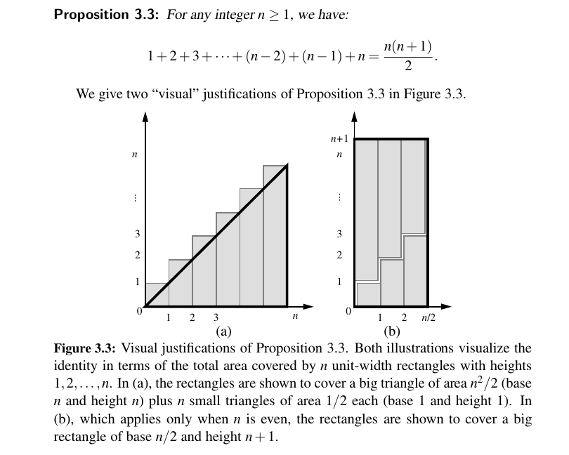
The quadratic function can also arise in the context of nested loops where the first iteration of a loop uses one operation, the second uses two operations, the third uses three operations, and so on.

That is, the number of operations is:

\[ 1 + 2 + 3 + · · · + (n − 2) + (n − 1) + n = \frac{n * (n-1)}{2} \]

Justification — Visuals help us understand.

The Cubic Function and Other Polynomials 😮¶

Continuing our discussion of functions that are powers of the input, we consider the cubic function, $f(n) = n^3$ which assigns to an input value $n$ the product of $n$ with itself three times.

The Exponential Function 😦¶

Another function used in the analysis of algorithms is the exponential function, $f(n) = b^n$ where $b$ is a positive constant, called the base, and the argument $n$ is the exponent.

That is, function $f(n)$ assigns to the input argument $n$ the value obtained by multiplying the base $b$ by itself $n$ times.

If we have a loop that starts by performing one operation and then doubles the number of operations performed with each iteration, then the number of operations performed in the nth iteration is $2^n$ .

Geometric Sums¶

Suppose we have a loop for which each iteration takes a multiplicative factor longer than the previous one.

This loop can be analyzed using the following proposition.

Everyone working in computing should know that $1 + 2 + 4 + 8 + · · · + 2^{n−1} = 2^n − 1$ for this is the largest integer that can be represented in binary notation using n bits.

These are called geometric summations, because each term is geometrically larger than the previous one if $a > 1$.

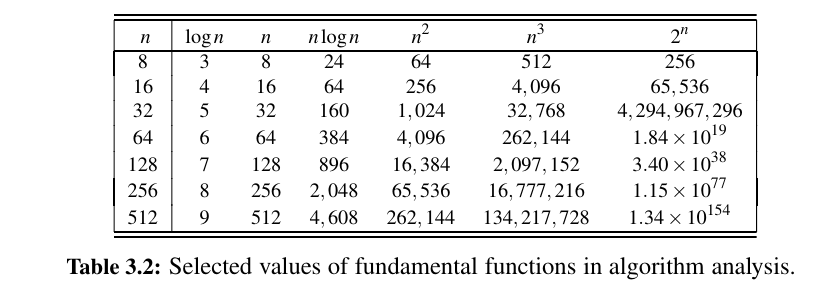
The Growth Rates¶

Here is all the functions we learned:

constant	log	linear	n log n	quadratic	cubic	exponential
`1`	`log(n)`	`n`	`n log(n)`	`n^2`	`n^3`	`a^n`

The Ceiling and Floor Functions¶

One additional comment is about floor and ceiling.

The analysis of an algorithm may sometimes involve the use of the floor function and ceiling function, which are defined respectively as follows:

ceil(x) = the largest integer less than or equal to x.
floor(x) = the smallest integer greater than or equal to x.

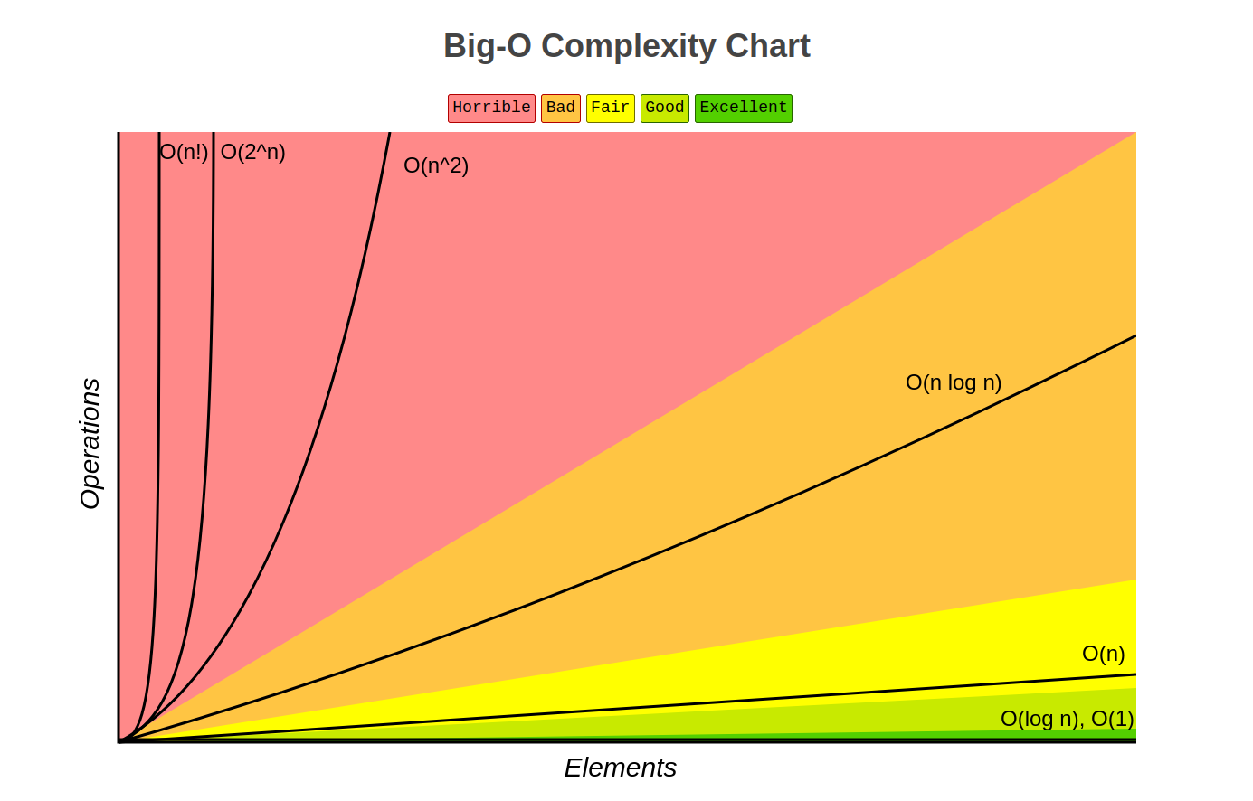
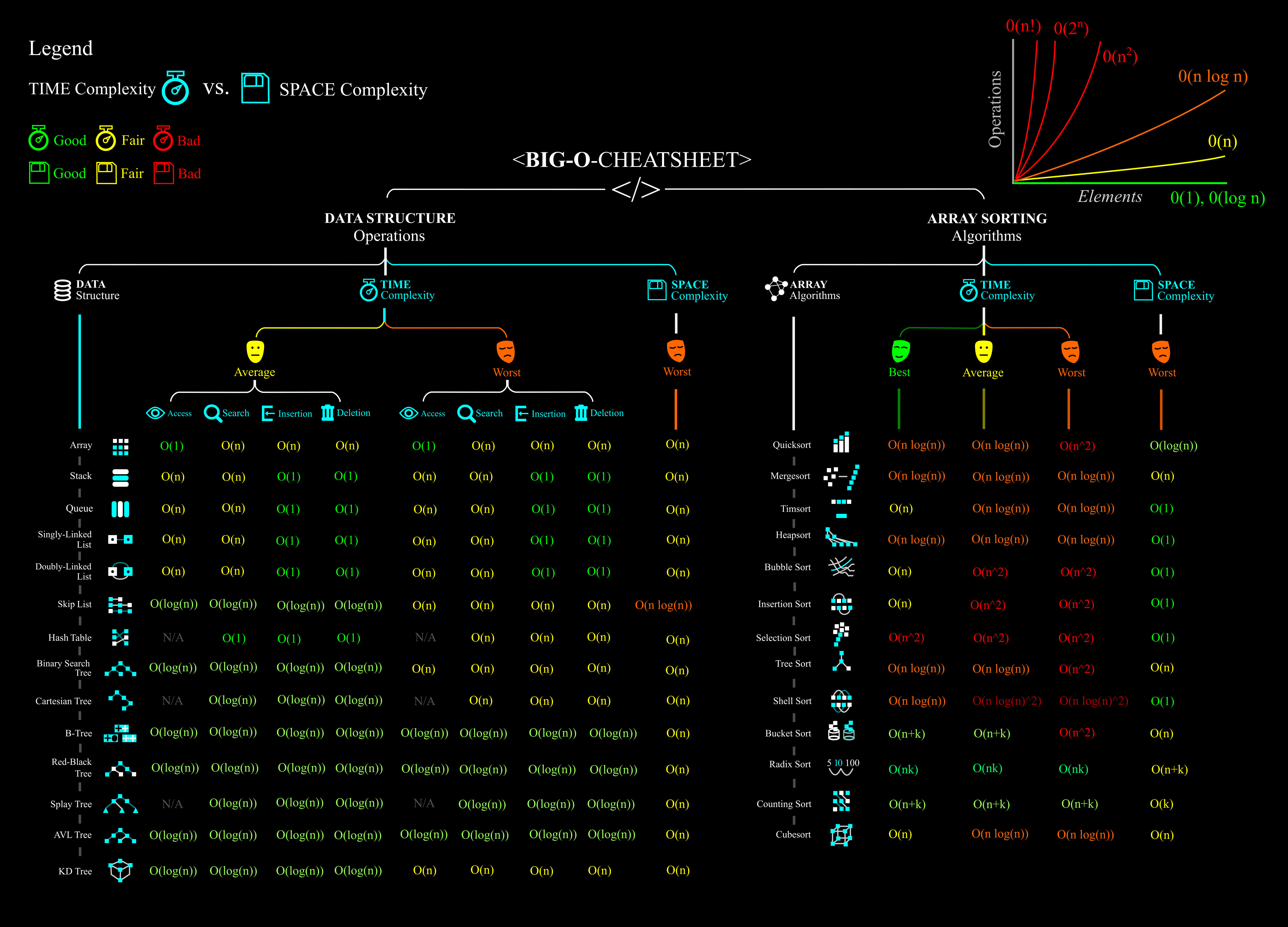
Here is a sneak peak for Data Structures coming up, from this wonderful 💚 source:

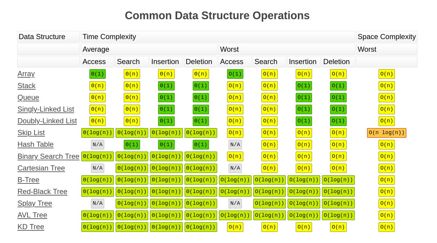
Even better, here is a poster that you can use: 💕

Asymptotic Analysis¶

In algorithm analysis, we focus on the growth rate of the running time as a function of the input size $n$, taking a “big-picture” approach.

For example, it is often enough just to know the running time of an algorithm grows proportionally to $n$. w We analyze algorithms using a mathematical notation for functions that disregards constant factors.

Namely, we characterize the running times of algorithms by using functions that map the size of the input, $n$, to values that correspond to the main factor that determines the growth rate in terms of $n$.

The “Big-Oh” Notation¶

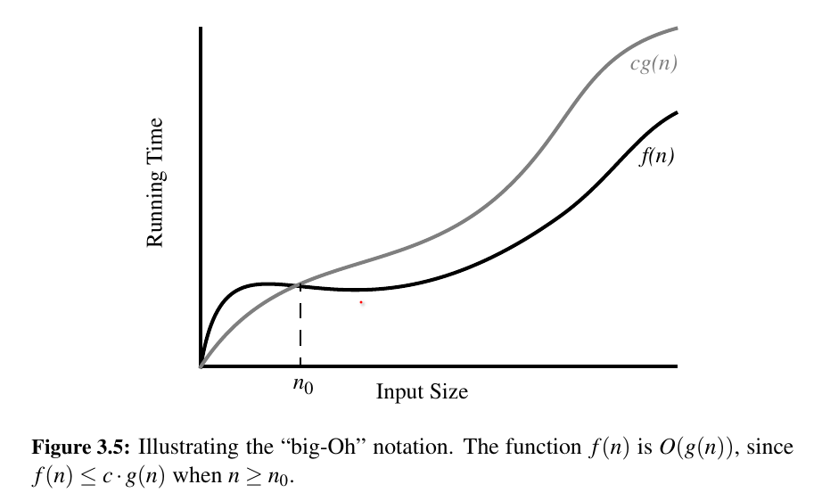
Let $f(n)$ and $g(n)$ be functions mapping positive integers to positive real numbers.

We say that $f(n)$ is $O(g(n))$ if there is a real constant $c > 0$ and an integer constant $n_0 ≥ 1$ such that $f (n) ≤ cg(n)$ for $n ≥ n_0$

This definition is often referred to as the “big-Oh” notation, for it is sometimes pronounced as “ $f (n)$ is big-Oh of $g(n)$."

The big-Oh notation allows us to say that a function $f(n)$ is “less than or equal to” another function $g(n)$ up to a constant factor and in the asymptotic sense as $n$ grows toward infinity.

def find_max(data):
    """Return the maximum element from a non empty Python List"""
    biggest = data[0]
    for val in data:
        if val > biggest:
            biggest = val
    return biggest

Using the big-Oh notation, we can write the following mathematically precise statement on the running time of algorithm find_max for any computer.

The algorithm, find_max, for computing the maximum element of a list of $n$ numbers, runs in $O(n)$ time.

The big-Oh notation allows us to ignore constant factors and lower-order terms and focus on the main components of a function that affect its growth.

\[ 5n^2 + 3 n * log n + 2n + 5 => O(n^2). \]

Big-Omega¶

Just as the big-Oh notation provides an asymptotic way of saying that a function is “less than or equal to” another function, the following notations provide an asymptotic way of saying that a function grows at a rate that is “greater than or equal to” that of another.

Let $f(n)$ and $g(n)$ be functions mapping positive integers to positive real numbers.

We say that $f (n)$ is $Ω(g(n))$, pronounced “$f(n)$ is big-Omega of $g(n)$" if $g(n)$ is $O(f(n))$, that is, there is a real constant $c > 0$ and an integer constant $n_0 ≥ 1$ such that $f(n) ≥ cg(n), \:for\:n ≥ n_0$

This definition allows us to say asymptotically that one function is greater than or equal to another, up to a constant factor.

Big-Theta¶

In addition, there is a notation that allows us to say that two functions grow at the same rate, up to constant factors.

We say that $f(n)$ is $Θ(g(n))$, pronounced “$f(n)$ is big-Theta of $g(n)$,” if $f(n)$ is $O(g(n))$ and $f(n)$ is $Ω(g(n))$ , that is, there are real constants $c' > 0$ and $c'' > 0$, and an integer constant $n_0 ≥ 1$ such that $c' g(n) ≤ f (n) ≤ c'' g(n)$ for $n ≥ n_0 $

Example 3.16:

\[ 3*n* (log n) + 4*n + 5 *(log n) \]

is

\[ Θ(n * log n) \]

Justification:

\[ 3*n*(logn) ≤ 3*n*(log n) + 4*n + 5 (log n) ≤ (3 + 4 + 5)* n *(log n) \\ for n ≥ 2 \]

Comparative Analysis¶

Between two algorithms solving the same problem, why wouldn't we want to choose the better one?

Function_growth — How fast can the functions grow?

Also, if you write "bad" code, code with worse asymptotical performance, you won't get very far even if you run it for a long time.

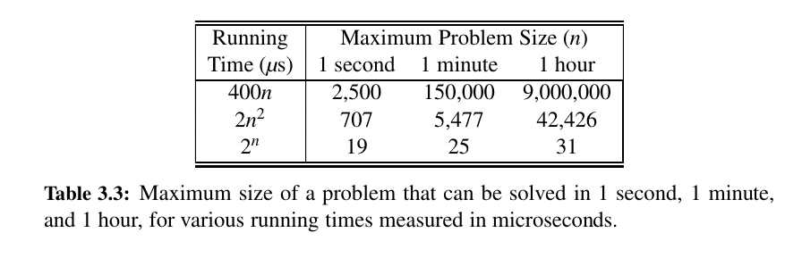
Tip

While it is true that the function $10^{100} n$ is $O(n)$, if this is the running time of an algorithm being compared to one whose running time is $10n log n$, we should prefer the $O(n log n)$ time algorithm, even though the linear-time algorithm is asymptotically faster.

Even when using the big-Oh notation, we should at least be somewhat mindful of the constant factors and lower-order terms we are “hiding.”

Examples of Algorithm Analysis:¶

Constant Time¶

Let's think of a list my_list = ["a", "b", "c"]

my_list[1] is $O(1)$, or len(my_list) is $O(1)$. Basically two accesses into memory.

Logarithmic Time¶

Binary Search is a great example for a $Olog(n)$ function

def binary_search(collection: list, target: int) -> int:
    """Find the index of target for non decreasing collection
    If target is not in the collection, return -1"""
    low, high = 0, len(collection) - 1
    while low <= high:
        middle = low + ((high - low) // 2)
        if target == collection[middle]:
            return middle
        elif target < collection[middle]:
            high = middle - 1
        else:
            low = middle + 1
    return -1

Linear Time¶

The find_max function was $O(n)$ as we have to traverse the collection once.

def find_max(col):
    """Find the maximum value in a given collection"""
    return max(col, key = float)

`n log n` Time¶

Classic sorts are $O(n(log n))$. Here is an example with heap sort using the Standard Library:

import heapq

def heap_sort(my_list):
    """Function to perform the sorting using heap sort"""
    heapq.heapify(my_list)  # the list is now a heap - O(n) time
    result = []
    while my_list:
        result.append(heapq.heappop(my_list)) # n times o(log(n))
    return result

col = [60, 20, 40, 70, 30, 10]
print("Input Array: ", col) # Input list: [60, 20, 40, 70, 30, 10]
print("Sorted Array: ", heap_sort(col)) # Sorted list: [10, 20, 30, 40, 60, 70]

If you cannot understand this right now, that is alright.

Just keep studying & getting better. 💕

`n^2` Quadratic Time¶

Here is a quadratic time algorithm:

def prefix_average1(s):
    """Return list such that for all j, A[j] equals avarage of s[0], ... s[j]"""
    n = len(s) # constant time
    A = [0] * n # o(n) time
    for j in range(n): # o(n^2)
        total = 0
        for i in range(j + 1):
            total += s[i]
        A[j] = total / (j + 1)
    return A

How about this?

def prefix_average2(S):
    n = len(S) # o(1)
    A = [0] * n # o(n)
    # o(n)
    for j in range(n):
        # o(n) - because of j + 1 time
        # The summation operation sum(S[0:j+1]) takes O(j+1) time
        # since it involves summing j+1 elements.
        A[j] = sum(S[0:j+1]) / (j + 1)
    return A

Although this looks like a better way, it still is $O(n^2)$

Here is one more approach (not even $O(nlogn)$, it is $O(n)$):

def prefix_average3(S):
    n = len(S) # o(1)
    A = [0] * n # o(n)
    total = 0 # o(1)
    for j in range(n): # o(n)
        # o(1)
        total += S[j]
        # o(1)
        A[j] = total / (j + 1)
    return A

In algorithm prefix_average3, we maintain the current prefix sum in a list A, effectively computing S[0] + S[1] + · · · + S[j]as total + S[j], where value total is equal to the sum S[0] + S[1] + · · · + S[j − 1] computed by the previous pass of the loop over j.

Just as a practice, here it is written again:

# what if we do not calculate the total over and over again?
def prefix_average_three(collection: list) -> list:
    a = [0] * len(collection)
    total = 0
    for i in range(len(collection)):
        total += collection[i]
        a[i] = total / (i + 1)
    return a

prefix_average_three([1,2,3,4,5]) # [1.0, 1.5, 2.0, 2.5, 3.0]

Here is another example, checking disjointedness in sets:

def disjoint1(A,B,C):
    for a in A:
        for b in B:
            for c in C:
                if a == b == c:
                    return False
    return True

This is clearly $o(n^3)$. Here is a better version.

def disjoint2(A,B,C):
    for a in A:
        for b in B:
            if a == b:
                for c in C:
                    if a == c:
                        return False
    return True

In the improved version, it is not simply that we save time if we get lucky.

We claim that the worst-case running time for disjoint2 is $O(n^2)$.

There are quadratic many pairs (a, b) to consider.

However, if A and B are each sets of distinct elements, there can be at most $O(n)$ such pairs with a equal to b. Therefore, the innermost loop, over C, executes at most $n$ times.

Here is another example, for whether all the elements in the given list are unique:

def unique1(S):
    for j in range(len(S)):
        for k in range(j+1,len(S)):
            if S[j] == S[k]:
                return False
    return True

Pretty clear that its $O(n^2)$. Here is a better way:

An even better algorithm for the element uniqueness problem is based on using sorting as a problem-solving tool.

In this case, by sorting the sequence of elements, we are guaranteed that any duplicate elements will be placed next to each other.

Thus, to determine if there are any duplicates, all we need to do is perform a single pass over the sorted sequence, looking for consecutive duplicates.

def unique2(S):
    temp = sorted(S)
    for j in range(1,len(temp)):
        if S[j-1] == S[j]:
            return False
    return True

The built-in function, sorted, produces a copy of the original list with elements in sorted order.

It guarantees a worst-case running time of $O(n log n)$, see Chapter 12 for a discussion of common sorting algorithms.

Once the data is sorted, the subsequent loop runs in $O(n)$ time, and so the entire unique2 algorithm runs in $O(n log n)$ time.

Simple Justification Techniques 🤔¶

Sometimes, we will want to make claims about an algorithm, such as showing that it is correct or that it runs fast. In order to rigorously make such claims, we must use mathematical language, and in order to back up such claims, we must justify or prove our statements.

By Example¶

“Every element x in a set S has property P.”

To justify that such a claim is false, we only need to produce a particular x from S that does not have property P. Such an instance is called a counterexample.

Example: Professor Amongus claims that every number of the form $2i − 1$ is a prime, when i is an integer greater than 1. Professor Amongus is wrong.

Justification: To prove Professor Amongus is wrong, we find a counterexample. Fortunately, we need not look too far, for $2^4 − 1 = 15 = 3 · 5$.

The “Contra” Attack¶

Another set of justification techniques involves the use of the negative. The two primary such methods are the use of the contrapositive and the contradiction.

Contrapositive¶

To justify the statement “if p is true, then q is true,” we establish that “if q is not true, then p is not true” instead. Logically, these two statements are the same, but the latter, which is called the contrapositive of the first, may be easier to think about.

Example: Let $a$ and $b$ be integers. If $a*b$ is even, then $a$ is even or $b$ is even.

Justification: To justify this claim, consider the contrapositive, “If a is odd and b is odd, then ab is odd.”

So, suppose $a = 2 j + 1$ and $b = 2k + 1$, for some integers j and k.

Then $a*b = 4 jk + 2 j + 2k + 1 = 2(2 jk + j + k) + 1$; hence, $a*b$ is odd.

Contradiction¶

Another negative justification technique is justification by contradiction, which also often involves using DeMorgan’s Law.

In applying the justification by contradiction technique, we establish that a statement q is true by first supposing that q is false and then showing that this assumption leads to a contradiction (such as $2 != 2$ or $1 > 3$).

By reaching such a contradiction, we show that no consistent situation exists with q being false, so q must be true. Of course, in order to reach this conclusion, we must be sure our situation is consistent before we assume q is false.

Example: Let a and b be integers. If ab is odd, then a is odd and b is odd.

Justification: Let $ab$ be odd. We wish to show that $a$ is odd and $b$ is odd. So, with the hope of leading to $a$ contradiction, let us assume the opposite, namely, suppose $a$ is even or $b$ is even.

In fact, without loss of generality, we can assume that a is even (since the case for b is symmetric).

Then $a = 2 j$ for some integer $j$. Hence, $ab = (2 j)b = 2( jb)$, that is, $ab$ is even.

But this is a contradiction: $ab$ cannot simultaneously be odd and even. Therefore, a is odd and b is odd.

Induction and Loop Invariants 🍓¶

This part can be understood from here.

Most of the claims we make about a running time or a space bound involve an integer parameter n (usually denoting an intuitive notion of the “size” of the problem).

Moreover, most of these claims are equivalent to saying some statement q(n) is true “for all n ≥ 1.” Since this is making a claim about an infinite set of numbers, we cannot justify this exhaustively in a direct fashion.

Induction¶

We can use induction when we want to show a statement is true for all positive integers n. (Note that this is not the only situation in which we can use induction, and that induction is not (usually) the only way to prove a statement for all positive integers.)

To use induction, we prove two things:

- Base case: The statement is true in the case where n = 1. 
- Inductive step: If the statement is true for n = k, then the statement is also true for n = k + 1.

This actually produces an infinite chain of implications:

- The statement is true for n = 1 
- If the statement is true for n = 1, then it is also true for n = 2 
- If the statement is true for n = 2, then it is also true for n = 3 
- If the statement is true for n = 3, then it is also true for n = 4 
- . . .

Together, these implications prove the statement for all positive integer values of n. (It does not prove the statement for non-integer values of n, or values of n less than 1.)

Loop Invariants¶

A loop invariant is a statement that we want to prove is satisfied at the beginning of every iteration of a loop.

In order to prove this, we need to prove three conditions: - Initialization: The loop invariant is satisfied at the beginning of the for loop. - Maintenance: If the loop invariant is true before the i'th iteration, then the loop invariant will be true before the i + 1st iteration. - Termination: When the loop terminates, the invariant gives us a useful property that helps show that the algorithm is correct.

Let's continue with Recursion! 🎋